Technical Report R-2017-1
Dr. Jerrold Prothero
[email protected]
Washington, D.C.
Last Update: February 28, 2017
Version 1.0
Copyright © 2017 Astrapi Corporation
Technology described in this document is covered by issued and pending Astrapi patents.
Table of Contents
Acknowledgment & Disclaimer
Abstract
1. Introduction
2. Mathematical Background
3. Instantaneous Spectral Analysis
Overview
Technical Description
Detailed Operations
Determine Signal Polynomial
Project Polynomial onto Cairns Series Functions
Convert from Cairns Series Functions to Cairns Exponential Functions
Combine Frequency Information
4.Waveform Bandwidth Compression
5. Spiral Polynomial Division Multiplexing
6. Single Spiral Modulation
7. Conclusion
Table of Tables
Table 1: Generalized Euler’s Term as a Function of m
Table 2: Number of Functions at Each m-Level
Table 3: The Cairns Series Coefficients
Table of Figures
Figure 1: First Eight Cairns Polynomials
Figure 1: Generation of Random Polynomial
Figure 2: Conversion to Taylor Polynomial
Figure 3: Zero Pad Taylor Polynomial
Figure 4: Normalization Coefficients
Figure 5: Generate Cairns Projection Matrix
Figure 6: Project Onto Cairns Space
Figure 7: Find Amplitude Values
Figure 8: Find Row Index
Figure 9: Sort Frequencies
Figure 10: Combine Amplitude Pairs
Figure 11: Reconstruction of Time Domain
Figure 12: ISA Time Domain and Frequency Domain Plots
Figure 13: Comparison of ISA and FT Spectral Usage
Technical Introduction to Spiral Modulation
Acknowledgment & Disclaimer
This material is based in part upon work supported by the National Science Foundation under Grant No. 1621082. Any opinions, findings, and conclusions or
recommendations expressed in this material are those of the author(s) and do not
necessarily reflect the views of the National Science Foundation.
Abstract
A unified introduction to spiral modulation is provided, including its underlying
mathematics and range of applications. Traditional digital telecommunication is
based conceptually on complex circles derived from Euler’s formula, leading to
transmission using sinusoids with constant amplitude over each symbol time.
Spectral information is analyzed using the Fourier Transform (FT), which averages
frequency information over a time interval. Spiral modulation is instead based on a
generalization of Euler’s formula, leading to a new technique called Instantaneous
Spectral Analysis (ISA) for representing signals as polynomials and converting them
into sinusoids with continuously-varying amplitude for transmission. ISA is also a
time-frequency analysis tool that makes it possible to describe the spectrum at a
particular point in time, not averaged over a time interval as with the FT. By for the
first time fully exploiting the capabilities of a nonstationary spectrum, spiral
modulation makes it possible to dramatically increase spectral efficiency, through
breaking an assumption in the sampling theorem that the spectrum is stationary.
Spiral modulation provides potential benefits that may include increasing data
throughput, reducing occupied bandwidth, reducing signal power, reducing latency,
and mitigating phase noise and coherent interference.
1. Introduction
This document is an introduction to spiral modulation intended for a technical audience with a strong background in telecommunications. For more detailed
information, which may be proprietary, please contact Astrapi.
Current digital communication has its foundations in 18th-century mathematics.
Conceptually, signals are defined by altering the parameters of complex circles, as
described by Euler’s formula. The transmission model is a sequence of constantamplitude sinusoids on a per-symbol basis, derived from complex circles. Spectral analysis is based on the Fourier Transform (FT), which uses Euler’s formula to convert a real-valued time sequence into a set of sinusoids each with constant
amplitude. Effectively, the FT averages frequency information over a time interval.
Spiral modulation is based on a 21st-century generalization of Euler’s formula that
describes spirals in the complex plane. When applied to digital communications, this
leads to a new technique called “Instantaneous Spectral Analysis” (ISA) that provides
a transmission model based on sinusoids with continuously-varying amplitude. ISA
also provides a tool for analyzing spectral information at each instant in time, not
averaged over a time interval as with the FT.
We will refer to a spectrum as “stationary” if its frequency information does not vary
over time, or equivalently if it is correctly represented by sinusoids with constant
amplitude. If this condition does not hold, the spectrum will be termed
“nonstationary”
The transition from circles to spirals is a conceptually simple change with remarkably profound implications for communications theory and practice. It has been said that “Custom is second nature often mistaken for first”, and in the same way characteristics of the mathematics we have applied to communications theory have often been accepted as inherent characteristics of communications itself.
Notably, the following statements often (although not universally) associated with
classical communication theory are affected significantly by spiral modulation.
- A real-valued time sequence has a unique spectral representation provided by the FT. The FT averages spectral information across a time interval, which implies that the spectrum is assumed to be stationary over that period. The well-established field of time-frequency analysis exists because this assumption is in practice at best a reasonable approximation. For spiral Technical Introduction to Spiral Modulation modulation, stationarity is a very poor approximation and examining its spectral content using an FT is inappropriate.
- Spectral occupancy should be measured in terms of FT roll-off. Since the FT is not an appropriate tool for analyzing nonstationary spectra, it is also not an
appropriate tool for measuring spectral occupancy if stationarity cannot be assumed. A spectral occupancy measure based on Inter-Channel Interference (ICI) is independent of a stationarity assumption and more economically meaningful. - Sampling at the Nyquist rate is sufficient to fully reconstruct a bandlimited signal. The Nyquist rate is a consequence of the sampling theorem, which cannot be proven without assuming the spectrum to be stationary. The
spectrum is never stationary for spiral modulation. - The Shannon-Hartley law is the upper bound on channel capacity. The proof of the Shannon-Hartley law requires the sampling theorem and therefore
implicitly assumes that the spectrum is stationary. - The brick wall filter in the frequency domain is equivalent to the sinc function in the time domain. This equivalence is a consequence of the FT. It therefore does not apply to cases in which the spectrum is not at least
approximately stationary. - A bandlimiting filter is necessary to constrain spectral occupancy. Spiral modulation transmitted using ISA is inherently characterized by a sharp upper bound on the frequencies into which it places power. It therefore may not require a filter to remove power above some frequency range, although filters may be desirable for other reasons.
The most interesting consequence of spiral modulation is that, by for the first time fully exploiting the capabilities of a nonstationary spectrum, it in principle provides a
means to exceed the Shannon limit on spectral efficiency. No traditional signal modulation technique based on sinusoids with constant amplitude over each symbol
time is capable of doing this.
Direct benefits of the dramatically higher spectral efficiency made possible by spiral
modulation include higher data throughput, lower signal power requirements, and
reduced spectral occupancy. Other potential benefits of spiral modulation include
lower latency and improved resistance to coherent interference and phase noise.
The following sections introduce the mathematical background and main
implementation paths for spiral modulation.
2. Mathematical Background
This section provides the core mathematical background necessary to understand
spiral modulation.
The familiar Euler’s formula
![]()
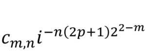
can be generalized by raising the imaginary constant 𝑖 on the left side to fractional powers. The new term
![]()
reduces to the standard Euler’s term in the special case 𝑚 = 2.
We can build the following table for positive integer values of 𝑚:
TABLE 1: GENERALIZED EULER’S TERM AS A FUNCTION OF M
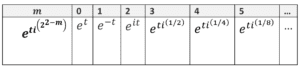
The standard Euler’s formula (2.1) can be proved by expanding 𝑒 𝑖𝑡 as a Taylor series and grouping real and imaginary terms. The same procedure can also be used for the term in (2.2) to derive a generalization of Euler’s formula for integer 𝑚 ≥ 0:
Where
![]()
The 𝜓𝑚,𝑛(𝑡) are called the “Cairns series functions” or the “Cairns polynomials”.
Notice that 𝜓2,0(𝑡) and 𝜓2,1(𝑡) give us the Taylor series for the standard cosine and
sine functions, respectively.
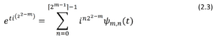
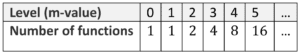
Each value of 𝑚 produces a “level” of functions 𝜓𝑚,𝑛(𝑡); from the summation limits
in Equation 2.3, it can be seen that each level has a total of ⌈2𝑚−1⌉ functions. That is:
TABLE 2: NUMBER OF FUNCTIONS AT EACH M-LEVEL
An important property of the 𝜓𝑚,𝑛(𝑡) is the regular pattern of their coefficients, as
shown in the below table.
TABLE 3: THE CAIRNS SERIES COEFFICIENTS
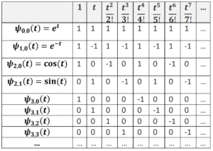
Here, the rows indicate the Taylor series coefficients for each 𝜓𝑚,𝑛(𝑡). For instance,
the row for 𝜓2,0(𝑡) = cos(𝑡) tells us that
From Table 4 it is easy to see, and not difficult to prove, that the 𝜓𝑚,𝑛(𝑡) coefficients define a set of orthogonal vectors. More precisely, if 𝑀 is a positive integer, then the
vectors formed from the first 2Μ coefficients of the functions 𝜓𝑚,𝑛(𝑡) for 0 ≤𝑚≤𝑀 constitute a set of orthogonal basis vectors for a2𝑀-dimensional space. These can be normalized to produce the orthonormal “2𝑀 Cairns basis vectors”.
The existence of the 2𝑀 Cairns basis vectors implies that any Taylor polynomial 𝑃 of
degree 𝑘<2𝑀 can be orthogonally projected onto polynomials formed from the first 2
𝑀 terms of the Cairns series functions simply by taking the inner product of 𝑃’s coefficients with the 2 𝑀 Cairns basis vectors. The resulting coefficients for each Cairns basis function are referred to as the “projection coefficients”.
The first 2𝑀 terms of the Cairns series functions 𝜓𝑚,𝑛(𝑡) are only an approximation
to the full infinite series expansion of the𝜓𝑚,𝑛(𝑡). However, the error in the approximation is 𝑂(𝑡(2𝑀)), with a reciprocal factorial coefficient, and therefore falls off very rapidly as 𝑀 increases. For high-degree polynomials, therefore, it is reasonable to speak of projecting onto the 𝜓𝑚,𝑛(𝑡) by this procedure.
It is well-known that the cosine and sine functions of Euler’s formula can be represented not only by Taylor series but also by sums of complex exponentials.
Explicitly:
![]()
and
This characteristic also holds for the generalized Euler’s formula. We can define.
By expanding the right side of Equation 2.8 as a sum of Taylor polynomials and
recursively cancelling terms, it can be shown that for all 𝑚 and 𝑛
𝐸𝑚,𝑛(𝑡) = 𝜓𝑚,𝑛(𝑡) (2.9)
Equation 2.9 tells us that once a polynomial has been projected onto the Cairns series functions, it can be immediately converted into a sum of complex exponentials. This is useful for converting a polynomial into sinusoids with continuously-varying amplitude, which is the basis for the ISA algorithm discussed
below.
As mentioned above, the Cairns basis functions allow any Taylor polynomial (which
includes any polynomial with terms having positive integer powers) to be projected
onto the Cairns series functions. Conversely, any weighted sum of Cairns series
functions corresponds uniquely to a particular Taylor polynomial. As described
below, Spiral Polynomial Division Multiplexing (SPDM) makes use of this fact in one
of its instantiations to compose and decompose sub-channels. In the most straightforward implementation, each sub-channel corresponds to one amplitude-modulated Cairns function 𝜓𝑚,𝑛(𝑡).
Let us look at the geometry of the generalized Euler’s term ![]() . By using the
. By using the
identity
![]() (2.10)
(2.10)
which is a special case of Euler’s formula, it follows that
![]() (2.11)
(2.11)
On the right side of Equation 2.11 the first factor,![]() , is a real-valued
, is a real-valued
exponential; the second factor, ![]() , describes a circle in the complex
, describes a circle in the complex
plane. Their product describes a spiral in the complex plane.
As shown above, 𝑚 = 0 generates the standard rising exponential; 𝑚 = 1 generates
the standard falling exponential; and 𝑚 = 2 generates the standard sine and cosine
functions.
From Equation 2.11 we can see that as 𝑚 increases above 𝑚 = 2, the rate of growth
increases and the rate of rotation decreases. In the limit as 𝑚 → ∞, ![]()
𝑡𝑖(22−𝑚) converges back to ![]() .
.
At every level of 𝑚, the 𝜓𝑚,𝑛(𝑡) share the growth and frequency properties of their
generating term ![]() . For instance, the Cairns functions with the fastest
. For instance, the Cairns functions with the fastest
rotation (and slowest growth) occur at 𝑚 = 2.
Another important observation is that for 𝑚 ≥ 2 Cairns functions with even 𝑛 are always symmetric around 𝑡 = 0, and Cairns functions with odd 𝑛 are always antisymmetric around 𝑡 = 0. This generalizes a well-known feature of the cosine and
sine functions.
The Cairns polynomials through 𝑚 = 3 are plotted below for the interval −3.1 ≤ 𝑡 ≤ 3.1.
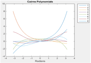
FIGURE 1: FIRST EIGHT CAIRNS POLYNOMIALS
3. Instantaneous Spectral Analysis
Overview
ISA converts a sequence of 𝑁 amplitude values (the “time domain”), or equivalently
a polynomial of degree 𝑁 − 1, into a sum of sinusoids with continuously-varying
amplitude. This is in contrast to the FT, which converts the time domain into a sum
of sinusoids with constant amplitude.
For a particular amplitude sequence, define 𝐵𝐹 to be the range of sinusoidal
frequencies occupied by the FT; let 𝐵𝐼 be the range of sinusoids with non-zero
power as generated by ISA.
Below are key differences between ISA and the FT.
- Since the FT represents an amplitude sequence with a basis set of sinusoids
having constant amplitude, it assumes an evaluation period over which the spectrum is stationary; that is, over which the power assigned to particular
frequencies is constant. This assumes that the source of the amplitude
sequence is Linear Time-Invariant (LTI). ISA does not require an LTI source. - The FT effectively averages spectral information over its evaluation period to
produce constant sinusoidal amplitudes. ISA is capable of determining
continuously-varying sinusoidal amplitudes at every instant in time (hence
the name “Instantaneous Spectral Analysis”). - For the FT, the maximum rate at which independent amplitude values can be
transmitted is equal to the Nyquist rate of 𝑓𝑁 = 2𝐵𝐹. For the ISA, there is no
inherent upper bound in terms of 𝐵𝐼 on the rate at which independent
amplitude values can be transmitted. ISA holds this advantage over the FT
because Shannon’s proof of the sampling theorem, from which the Nyquist
rate derives, assumes that the spectrum is stationary over the evaluation
interval. ISA violates this assumption. - Stating the above point in a different way, using ISA it is possible to transmit
a sequence of amplitude values in a given amount of time using a dramatically smaller range of frequencies with nonzero amplitude than is possible with the FT representation. - Effectively, for a given amplitude sequence time duration, the FT responds to
a higher level of detail in the amplitude sequence by utilizing higher frequencies (increasing 𝐵𝐹). ISA responds by increasing the density of sinusoids within a constant 𝐵𝐼.
We are used to referring to the output of the FT as the frequency domain, but really
it is a frequency domain; it provides a possible representation of the time domain in
terms of sinusoids with constant amplitude. ISA provides a different frequency domain representation in terms of sinusoids with continuously-varying amplitude.
This raises the question of how we should think about occupied bandwidth: is the FT
representation of occupied bandwidth “correct”, or is the ISA representation
“correct”?
The answer is that it depends on how the signal was generated. If the source was LTI
over the evaluation interval, then the FT representation is correct.
However, ISA provides a recipe for generating a non-LTI signal source that will
dramatically reduce the necessary range of frequencies with nonzero amplitude
necessary for transmission; for such a source, the FT representation is incorrect.
Using ISA, a sequence of amplitude values can be transmitted such that the product
of the bandwidth 𝐵𝐼 (defined in terms of the range of frequencies containing nonzero power) times the signal duration time T is always equal to one. Since a polynomial of degree D corresponds to D+1 independent amplitude values, this makes it possible to exceed the Nyquist rate. This occurs because the proof of the sampling theorem, from which the Nyquist rate derives, assumes that the spectrum is stationary over the evaluation interval. ISA violates this assumption.
Practically, bandwidth measurement matters because it affects how closely channels
can be packed together without Inter-Channel Interference (ICI). The real test of ISA
bandwidth efficiency is the extent to which it allows for closer channel packing.
Technical Description
The key steps of ISA are as follows.
- Represent a signal as a polynomial. This can occur either by fitting a polynomial to a sequence of amplitude values, or by selecting or generating the signal polynomial directly. This topic is covered in more detail in the sections below on Waveform Bandwidth Compression (WBC) and Spiral Polynomial Division Multiplexing (SPDM).
- Project the signal polynomial onto the Cairns series functions 𝝍𝒎,𝒏(𝒕). The projection occurs in the polynomial coefficient space.
- Convert from the Cairns series functions 𝝍𝒎,𝒏(𝒕) to the Cairns exponential functions 𝑬𝒎,𝒏 (𝒕). This is simply a labelling change as the two representations are equivalent numerically; however, the Cairns exponential
functions provide frequency information explicitly that is implicit in the
Cairns series functions. - Combine frequency information contained within the Cairns exponential functions. Group terms with the same frequencies to provide a
representation of the signal polynomial in terms of a sum of sinusoids with
continuously time-varying amplitudes.
The mathematics for the second and third steps were provided in 2. Mathematical
Background. A description of the fourth step, and MATLAB® software for all four
steps, is provided here.
While spectral usage is not readily apparent from the 𝜓𝑚,𝑛(𝑡) representation, it can
be determined precisely, and on an instant-by-instant basis, from the equivalent 𝐸𝑚,𝑛(𝑡). Essentially, projection onto 𝜓𝑚,𝑛(𝑡) allows us to decompose a polynomial, and then representing it as 𝐸𝑚,𝑛 (𝑡) allows us to generate an equivalent set of sinusoids with continuously-varying amplitude.
Each 𝐸𝑚,𝑛
(𝑡) can be expressed as a sum of products in which each term is the product of a phase-adjusted real-valued exponential with a complex circle. The real-valued exponentials may be either rising or decaying, and may have different growth constants in the exponent. The complex circles may rotate in either direction, and
with different frequencies.
By viewing the real-valued exponentials as continuously time-varying coefficients
applied to sinusoids, we have an approach to defining instantaneous spectrum. At
any particular time, the sum of the real-valued exponentials applied to complex circles of the same frequency defines the spectral usage at that particular frequency
at that particular time.
In more detail, by using the Euler’s formula identity ![]() = 𝑖 it is possible to
= 𝑖 it is possible to
represent 𝐸𝑚,𝑛(𝑡) as
![]()
![]()
![]()
In the above equation, the phase is determined by ![]() , the amplitude
, the amplitude
by ![]() , and the frequency by
, and the frequency by ![]() .
.
The instantaneous spectral information can be found by summing the phase weighted-amplitude information associated with each frequency.
Note the following points:
- For 𝑚 = 0 and 𝑚 = 1 the frequency factor is equal to the constant 1
- For 𝑚 ≥ 2, no two distinct 𝑚 levels will contain the same frequencies, since
sin depends on 𝑚.
 - The same frequency appears in for every 𝑛 at level 𝑚, since
sin does not depend on 𝑛.
Since both sin and cos can switch signs depending on the value of 𝑝, it follows that for 𝑚 ≥ 2 each positive frequency will be matched by an equal negative frequency, and that for 𝑚 ≥ 3 each positive and negative frequency will appear with both a rising and falling exponential as its real-valued amplitude coefficient.
To find the instantaneous amplitude of each frequency, we have to algebraically
assemble all terms that have the same frequency. Since (as noted above) the
frequency factor does not depend on 𝑛, the same frequency information will appear
in all ![]() functions having the same 𝑚. We therefore have to sum phase adjusted terms across 𝑛 values at the same 𝑚 level.
functions having the same 𝑚. We therefore have to sum phase adjusted terms across 𝑛 values at the same 𝑚 level.
Since a particular frequency is fully-determined by the combination of its 𝑚 and 𝑝
values, let us denote a given frequency by𝑓𝑚,𝑝 and its amplitude at a particular time
by ![]() . Then we have
. Then we have
![]()
![]()
This equation provides the instantaneous frequency amplitudes associated with the
polynomial 𝑃 at every distinct time 𝑡 over its evaluation interval. As noted above, for
𝑚 ≥ 3 each frequency will appear twice, associated with each of a rising and
decaying exponential amplitude. These paired amplitudes should be summed
together. A detail is that the 𝑐𝑚,𝑛 were found by projecting Taylor coefficients onto the 𝜓𝑚,𝑛(𝑡) normalized by their number of non-zero terms. However, ![]() reconstructs the signal polynomial from
reconstructs the signal polynomial from ![]() terms that have not been normalized in this way. Since
terms that have not been normalized in this way. Since ![]() =
= ![]() the same projection normalization factor as applied to the
the same projection normalization factor as applied to the ![]() must be applied for matched 𝑚, 𝑛 values; this was left out for readability but is performed in the below software.
must be applied for matched 𝑚, 𝑛 values; this was left out for readability but is performed in the below software.
Detailed Operations
The below subsections provide detailed operations for the corresponding high-level steps given above.
Determine Signal Polynomial
As discussed above, a signal can be viewed as equivalent to a polynomial or sequence of polynomials. A polynomial for signal transmission can arise either from fitting a polynomial to a sequence of data-carrying amplitude values, or by generating the polynomial directly, as described in the WBC and SPDM sections below.
Assuming the signal is given to us as a sequence of real-valued amplitude values, standard techniques exist for fitting a polynomial to the sequence of signal amplitude values, and others are currently under investigation at Astrapi. ISA does not depend on which method is used. Usual considerations apply, such as whether to produce a high-order polynomial that exactly fits the data sequence, or a lowerorder polynomial that is an adequate fit but perhaps better captures the underlying pattern. The only concern for ISA is that a polynomial be provided that represents
the time domain amplitude sequence.
For illustrative purposes, the following figure provides MATLAB code to generate a polynomial of arbitrarily chosen 25th degree, with random Taylor coefficients between -10 and 10.
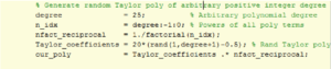
FIGURE 2: GENERATION OF RANDOM POLYNOMIAL
Project Polynomial onto Cairns Series Functions
This operation converts a polynomial 𝑃 representing the signal time-domain data
into a weighted sum of Cairns series functions.
First, we convert 𝑃 into a Taylor polynomial by multiplying through by the factorial
of each term’s power. In the below MATLAB code sample, a polynomial is
represented as a row vector of coefficients called poly_coefficients, with the highest
power on the left. The resulting Taylor_coefficients represents the same polynomial
with the factorials implicit.
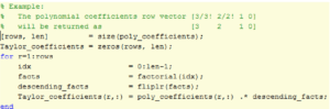
FIGURE 3: CONVERSION TO TAYLOR POLYNOMIAL
The code in Figure 3: Conversion to Taylor Polynomial is capable of handling a matrix in which each row represents a distinct polynomial, although for current purposes a single row is sufficient.
To shorten the notation, we refer to “Taylor_coefficients” equivalently as “Taylor_vec” below.
Next, if necessary we pad “Taylor_vec” with minimum-value high-term coefficients
so that the number of coefficients is a power of two, i.e. 2 𝑀 for positive integer 𝑀. This is because our polynomial coefficient projection is based on a table with a power-of-two number of rows and columns.
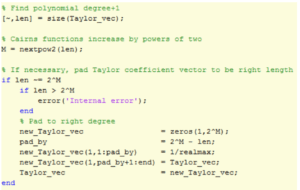
FIGURE 4: ZERO PAD TAYLOR POLYNOMIAL
We next construct the Cairns projection matrix
The following MATLAB code finds the normalization coefficient for each row of the
Cairns projection matrix.
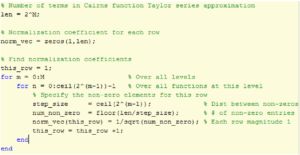
FIGURE 5: NORMALIZATION COEFFICIENTS
Given the normalization coefficients, the following code generates the Cairns
projection matrix.
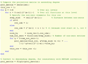
FIGURE 6: GENERATE CAIRNS PROJECTION MATRIX
Given the Cairns projection matrix, our Taylor polynomial can be projected onto
Cairns space by simple matrix multiplication. The following code produces a row
vector in which each row is the coefficient for a Cairns series function.
![]()
FIGURE 7: PROJECT ONTO CAIRNS SPACE
Convert from Cairns Series Functions to Cairns Exponential Functions
Because of the identity ![]() =
= ![]() , the conversion from Cairns series functions to Cairns exponential functions is automatic. We simply consider the projection coefficient for each
, the conversion from Cairns series functions to Cairns exponential functions is automatic. We simply consider the projection coefficient for each ![]() to be applied to the corresponding
to be applied to the corresponding ![]() .
.
However, because each ![]() was normalized as described above, the same normalization factors must be applied to the
was normalized as described above, the same normalization factors must be applied to the ![]() . In the below code, these normalization coefficients are held in the proj_norm row vector.
. In the below code, these normalization coefficients are held in the proj_norm row vector.
Combine Frequency Information The below code shows how to combine amplitude information associated with each frequency by summing across ![]() 𝑛-values. Note that the amplitudes are time-dependent (specified by the evaluation time 𝑡).
𝑛-values. Note that the amplitudes are time-dependent (specified by the evaluation time 𝑡).
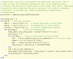
FIGURE 8: FIND AMPLITUDE VALUES
The function mn_to_row_index converts from a pair of 𝑚, 𝑛 values to the corresponding matrix index. It was given in-line in Figure 6: Generate Cairns Projection Matrix above, and is defined as follows.
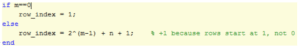 FIGURE 9: FIND ROW INDEX
Frequency values across 𝑚-levels are interleaved, so next we sort.
![]()
FIGURE 10: SORT FREQUENCIES
We now add for each frequency the rising and decaying exponential amplitudes. In
the process, the frequency vectors are shortened.
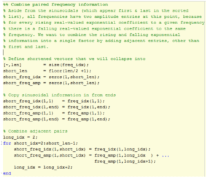
FIGURE 11: COMBINE AMPLITUDE PAIRS
We now have the instantaneous frequency and amplitude information stored in
short_freq_idx and short_freq_amp respectively.
The last step is to show how the instantaneous spectral information found above
can be used to reconstruct the time domain at a particular time value t.
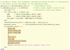
FIGURE 12: RECONSTRUCTION OF TIME DOMAIN
The accuracy of the reconstruction increases with the degree of the polynomial
representing the signal, since the projection onto Cairns space becomes more
precise with longer polynomials. For instance, for a random 25th-degree polynomial
maximum percentage reconstruction ratio errors are less than ![]() .
.
The left panel of the following figure shows the time domain for a random 15th
degree Taylor polynomial (solid red line) and its five positive-frequency ISA
components traced over time (dashed red lines).
The right panel of the figure shows the ISA sinusoidal amplitudes for matched
positive and negative frequencies at the arbitrarily-chosen time of 𝑡 = 0.20.
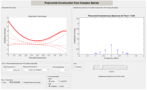
FIGURE 13: ISA TIME DOMAIN AND FREQUENCY DOMAIN PLOTS
In this case, the maximum ratio percentage error in the ISA reconstruction of the
polynomial across the entire evaluation interval is ![]() ; the mean percent
; the mean percent
reconstruction error is ![]() . The accuracy of the ISA reconstruction
. The accuracy of the ISA reconstruction
improves as the polynomial degree increases, since longer Taylor series are used.
Notice that the simulated transmission time duration Τ is 1 microsecond, and the
range of frequencies B in which ISA puts power is exactly 1 MHz. Since a random 15th degree polynomial transmits 16 independent amplitude values, the number of
amplitude values that can be transmitted in this way is 16𝐵𝑇. This is 8 times higher
than the 2𝐵𝑇 limit provided by the sampling theorem on the assumption (which ISA
breaks) that the spectrum is stationary over the transmission interval.
This difference is apparent from comparing the mean ISA spectral power with the FT
of the amplitude sequence generated by the random 15th degree polynomial, as displayed below.
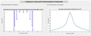
FIGURE 14: COMPARISON OF ISA AND FT SPECTRAL USAGE
In this figure, as shown in the left panel all ISA power is placed within the 1MHz
range. The FT in the right panel is on a frequency larger scale, showing only a
roughly 35dB roll-off at 10MHz.
4.Waveform Bandwidth Compression
The ISA algorithm detailed above gives us the ability to transmit signals using
sinusoids with continuously-varying amplitude, rather than the traditional sinusoids
with constant amplitude per symbol time. Doing so potentially allows data
throughput to be increased by transmitting independent amplitude values at a rate
higher than the Nyquist rate. As discussed above, this is possible because the proof
of the sampling theorem rests on an assumption that the spectrum is stationary,
which ISA violates.
Waveform Bandwidth Compression (WBC) arises from asking the question: “What is
the simplest way to obtain benefits from ISA while changing existing radio architecture as little as possible?” The WBC answer is to intervene in the encoder of
traditional signal modulation methods such as Phase-Shift Keying (PSK) or Quadrature Amplitude Modulation (QAM).
Any digital signal modulation technology produces a sequence of data-carrying
amplitude values that it intends to transmit using sinusoids. WBC views that
sequence of amplitude values as defining a sequence of polynomials of some
degree. Applying ISA then makes it possible express the data-carrying amplitude
values into a much smaller range of frequencies with nonzero amplitude than would
be necessary using traditional methods. This has the effect of compressing the
waveform bandwidth. In principle, the receiver design is not affected by WBC
because the expected sequence of amplitude values arrives, although expressed
differently in terms of sinusoidal sums.
A rough analogy, for purposes of building intuition, is that the same shape Chinese
parade dragon can be produced with more or less people underneath, depending on
how the people are deployed. In a similar way, WBC can deliver the same sequence
of amplitude values as traditional transmission using a smaller range of nonzero
frequencies, by deploying the frequencies differently (exploiting continuous
sinusoidal amplitude variation).
For further details on WBC, please contact Astrapi.
5. Spiral Polynomial Division Multiplexing
WBC, discussed above, provides a minimally-invasive approach to applying ISA to
traditional radio architecture. Spiral Polynomial Division Multiplexing (SPDM) takes a different approach. SPDM arises from asking the question: “If we were going to
design radio communications from scratch using ISA, what would we do?”
Since ISA potentially provides us for the first time with a bandwidth-efficient means
to transmit arbitrary polynomials, it opens the possibility of designing a communication system to use a basis set of polynomials for its symbol waveforms.
The SPDM model is that data is encoded using amplitude modulation of a basis set
of polynomials, and transmission occurs using ISA. This provides a very natural link
between digital data and analog waveform transmission. Every polynomial of degree
𝐷 is equivalent to a sequence 𝐷 + 1 independent amplitude values. The polynomial
itself describes an analog waveform suitable for transmission using ISA; the value of
the polynomial sampled at specified times can convey digital data.
Since general polynomials have much more waveform distinguishability than the
sinusoids used by traditional signal modulation methods, they are more resistant to
noise, and therefore may have much better Bit Error Rate (BER) performance as a
function of ![]() .
.
Within the SPDM broad umbrella are a number of topics.
- Choice of basis polynomials. A straight-forward implementation of SPDM
is to amplitude-modulate a basis set of Cairns polynomials, although other polynomial basis sets are also possible. For instance, to convey 8 bits per symbol (comparable to 256-QAM), one could support two amplitude levels for each of eight basis polynomials. An 8-bit sequence is then transmitted by producing a “transmission polynomial” corresponding to the weighted sum of the basis polynomials, and generating a sequence of amplitude values from the transmission polynomial. The task of the receiver, given a sequence of amplitude values, is to determine the polynomial that generated the sequence, and therefore the transmitted message. - Signal detection algorithm. The receiver can use standard minimum
Euclidean distance signal detection, and/or other techniques arising from
the properties of the polynomial basis set. - Synchronization. The use of polynomials provides new capabilities for
synchronization, which are the subject of National Science Foundation
(NSF)-funded research. - Single or multi-user configurations. Different communication subchannels can optionally be assigned to subsets of the polynomial basis set
that is combined into the transmission polynomial (hence the “Division
Multiplexing” in SPDM). - Coherent interference rejection. To the extent that coherent interference
can be described by a set of polynomials, linear algebra can potentially be
applied to generate an SPDM polynomial basis set that is orthogonal to
the coherent interference, thus mitigating its effect.
Potential benefits of SPDM include
- Much better BER vs. 𝑬𝒃/𝑵𝟎 performance than traditional signal
modulation techniques such as QAM, due to the much greater symbol
waveform distinguishability of general polynomials compared to simple
sinusoidal modulations. - Bandwidth-efficient transmission using ISA.
- Less vulnerability to phase noise since SPDM does not explicitly encode
information into phase. - Less vulnerability to coherent interference due to new SPDM-specific
mitigation techniques involving rotation of the basis polynomial set. - Lower signal power requirements since the higher spectral efficiency of
SPDM can be used to reduce signal power, for the same communication
performance. - Lower latency since SPDM spectral efficiency can be used to reduce
Forward Error Correction (FEC) overhead.
For further details, please contact Astrapi.
6. Single Spiral Modulation
The primary focus of this document has been on ISA-based techniques that exploit
sums of complex spirals. However, a more basic approach is also possible, which modulates the generalized Euler’s term in much the same way that traditional signal
modulation uses the standard Euler’s term, but with an extra parameter related to
the continuous complex amplitude variation of a spiral.
ISA as described in previous sections makes use of an integer-valued 𝑚 parameter.
However, we can replace this with a real-valued 𝑔 parameter, and we can treat 𝑔 as
a parameter that can be modulated.
![]()
Fixing 𝑔 = 2 would give us the standard Euler’s formula and support standard
techniques such as amplitude and phase modulation. Allowing 𝑔 to take on values
other than 2 opens a means to modulate spiral waveform shape. Other ways of
modulating spiral waveform shape are also possible, notably controlling the spiral
complex amplitude using splines to smooth discontinuities.
It is generally useful to return the complex amplitude to its original value at the end
of each symbol time, to minimize discontinuities. This involves a “ramping up” and
“ramping down” period (or the reverse).
When compared to a comparable PSK implementation, one advantage of single
spiral modulation can be much faster side-lobe roll-off as measured using a
traditional FT, since intra-symbol discontinuities can be reduced by assigning a low
complex amplitude to the inter-symbol boundary.
There are other possible benefits of single-spiral modulation, including the ability to
send reference signal information that also carries traffic.
For further details, please contact Astrapi
7. Conclusion
Astrapi has pioneered a new form of communication based on complex spirals,
rather than the traditional complex circles. Based on a solid mathematical foundation and for the first time fully exploiting the capabilities of a nonstationary
spectrum, spiral modulation potentially opens the door to a range of benefits
centered around higher spectral efficiency. The ability to exploit a much wider
symbol waveform design space based on polynomials also makes available new
techniques for coherent interference rejection and other benefits.