![]()
Dr. Jerrold Prothero
[email protected]
Washington, D.C.
May 2, 2012
Copyright © 2012 Astrapi Corporation
Technical Report
Table of Contents
Abstract
1. Introduction
2. The Frequency of Definition
3. Power and Signal Distance
4. Non-Periodic Channel Capacity
5. Conclusion
Appendix A: Introduction to Cairns Space
Appendix B: The Generalized Euler’s Formula Expressed as Series Functions
Appendix C: The Equivalence of the Cairns Series and Exponential Functions
Abstract
Shannon’s law for the information-carrying capacity of a noisy channel is generally
assumed to apply to any possible set of signals. However, since his proof requires Fourier analysis to establish the Nyquist rate and the signal distance formula, the domain of applicability for Shannon’s law is restricted to signals based on the periodic functions. This technical report derives a generalization of Shannon’s law
for signals based on non-periodic functions. Non-periodic signals are shown to be
able to store information in both frequency and exponential growth parameters. The
effect is that non-periodic channel capacity is not fully determined by the available
bandwidth and the signal-to-noise ratio, as in the periodic case. Channel capacity
can be increased beyond the periodic Shannon limit provided that the communication system can support a sufficiently high slew rate and sampling rate.
1.Introduction
Claude Shannon’s 1949 paper on communication over noisy channels¹ established an upper bound on channel information capacity, expressed in terms of available bandwidth and the signal-to-noise ratio. This is known today as Shannon’s law, or the Shannon-Hartley law.
In proving his law, Shannon made use of Fourier analysis to establish the Nyquist
rate and the signal distance formula. Since the domain of applicability of Fourier
analysis is the periodic functions, the proof developed by Shannon for Shannon’s law
strictly only applies to signals based on periodic functions (characterized by returning to the same amplitude values at regular time intervals) and does not
necessarily extend to non-periodic functions. This limitation is much more restricting than is generally realized.
The fact that Fourier analysis is limited to periodic functions can be understood
technically in terms of its fundamental operations: if the periodicity constraint is
violated then orthogonality fails, in which case the Fourier coefficients share
overlapping information. While Fourier analysis may work reasonably well for
approximately periodic functions, it is increasingly and inherently less reliable as the
departure from periodicity increases.
However, it is more useful for current purposes to understand the limitations of
Fourier analysis in a more intuitive sense. The fundamental assumption made by
Fourier analysis is that it is possible to cleanly separate the time domain from the
frequency domain: that is, that the time-domain information can be represented
using frequency components with constant (i.e., not time-varying) amplitude.
Perhaps the simplest example of a (non-periodic) function that breaks the Fourier
model is a spiral. Suppose we start with circular motion at constant angular speed in
the complex plane. Next, increase the amplitude of the circle continuously overtime
to produce a spiral. By the definition of frequency (the reciprocal of the time
necessary to travel an angular distance of two pi), the spiral and the original circle
have the same frequency.
However, Fourier analysis is unable to correctly identify the spiral as having the
same frequency profile as the circle. The reason is that the spiral lacks a constant frequency amplitude coefficient. It is not possible to represent spirals in terms of
frequency components that do not vary with time.
Seen in this light, Fourier analysis is limited to functions constructed from the special case of spirals that have constant amplitude (which is to say, circles). Since
unrestricted spirals are much more general than circles, it is apparent that the
restriction of Fourier analysis to periodic functions is a quite significant limitation.
This consideration directly affects the scope of Shannon’s law as it may apply to nonperiodic functions.
Because deployed signal modulation techniques have been based on cosine and sine
waves, which are periodic, the limitation of Shannon’s law to periodic functions has
not previously been of practical importance. However, Astrapi’s Compound Channel
Coding™ (cCc™) signal modulation is based instead on highly non-periodic spirals. It is therefore necessary to generalize Shannon’s law to cover non-periodic functions.
That is the task of this technical report.
There are two main problems addressed by this report, which may be thought of as
addressing signal “time” and “space”. The “time” problem is to determine the
necessary sampling rate to reconstruct non-periodic signals. The “space” problem is
to determine the degree to which signals can be made “distant”, or distinguishable
from each other, subject to power constraints. Combining the solutions to these
problems determines the information capacity for channels with non-periodic
signals.
2. The Frequency of Definition
Shannon’s proof establishes that signals based on periodic functions can be
reconstructed with complete accuracy by sampling at twice the highest baseband
frequency contained in the signal. This is now known as the “Nyquist frequency”,
denoted ![]() .
.
The task of this section is to establish a generalization of ![]() for non-periodic signals.
for non-periodic signals.
To do this, it is useful to introduce the concept of “frequency of definition”.
Definition: The “frequency of definition”, ![]() , is specified to be the minimum
, is specified to be the minimum
sampling rate necessary to fully reconstruct the (in general, non-periodic) signal
transmitted through a bandlimited channel.
It is also useful to make a distinction between channels that support only periodic
waveforms (Shannon’s implicit assumption) and more general channels.
Definition: A “periodic channel” is a communication channel that supports only
periodic waveforms.
Definition: A “non-periodic channel” is a communication channel that supports both non-periodic and periodic waveforms (with periodic waveforms a limiting special case of non-periodic waveforms).
Clearly, for periodic channels we must have ![]() . However, for non-periodic
. However, for non-periodic
channels we will see that it is possible to have ![]() . This has the effect of increasing the channel capacity beyond the limit Shannon envisioned.
. This has the effect of increasing the channel capacity beyond the limit Shannon envisioned.
The central result of this section is encapsulated in the following theorem.
Theorem 1 (“Frequency of Definition”): For a non-periodic channel, no finite upper limit is placed on the frequency of definition ![]() by the available bandwidth W.²
by the available bandwidth W.²
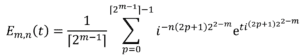
The proof of Theorem 1 can be approached by posing the following problem.
Suppose that our channel’s baseband frequency range is bounded by . Represent
the signal as a series of polynomials of degree , each running from
![]() (2.1)
(2.1)
which may be denoted ![]() . What is the maximum polynomial degree K that can be transmitted without loss of information?
. What is the maximum polynomial degree K that can be transmitted without loss of information?
There is an equivalence relationship between and . A ![]() -degree polynomial
-degree polynomial
requires K + 1 independent sample points to be specified uniquely. Conversely, if K + 1 independent sample points are available, they uniquely define a polynomial
of degree K . This leads to the following equation:
![]() (2.2)
(2.2)
It is therefore possible to prove Theorem 1 by proving that there is no upper bound
on K for a bandlimited non-periodic channel.
Note that the Nyquist rate tells us that
![]() (2.3)
(2.3)
and therefore K = 1 for periodic channels.
Let us now consider what it means for a polynomial![]() to be transmitted without loss of information over a non-periodic channel with baseband bandwidth W. Assuming perfect bandlimiting,
to be transmitted without loss of information over a non-periodic channel with baseband bandwidth W. Assuming perfect bandlimiting,
can be transmitted without loss of information ![]() if it can be constructed from component waveforms that make no use of frequencies greater than W . Conversely, if any component waveform uses a frequency greater than W, then
if it can be constructed from component waveforms that make no use of frequencies greater than W . Conversely, if any component waveform uses a frequency greater than W, then ![]() cannot be transmitted without loss of information.
cannot be transmitted without loss of information.
We now prove by construction that for a non-periodic channel it is always possible
to build ![]() from component waveforms that make no use of frequencies greater than W.
from component waveforms that make no use of frequencies greater than W.
The proof makes use of the idea of Cairns space, which was introduced previously.³
However, all relevant material is provided in the appendices, so as to make this
technical report self-contained.
The key steps of the proof are as follows.
- Project the
 onto the Cairns space series functions .
 - Convert from the series representation to the equivalent exponential representation .
- Show that in the exponential representation, the frequency range can be made arbitrarily narrow.
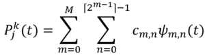
Assume without loss of generality that the ![]() are represented as Taylor polynomials. (This is merely a choice of how the polynomial coefficients are represented.) Then
are represented as Taylor polynomials. (This is merely a choice of how the polynomial coefficients are represented.) Then![]() can be represented as a weighted sum of Cairns series functions, found by orthogonal projection of the
can be represented as a weighted sum of Cairns series functions, found by orthogonal projection of the ![]() coefficients, as described in Appendix A. That is, there is some set of constants
coefficients, as described in Appendix A. That is, there is some set of constants ![]() such that
such that
 (2.4
(2.4
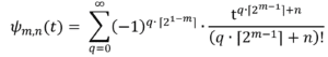
where
![]() (2.5)
(2.5)
Once ![]() has been expressed as Cairns series functions through Equation 2.4, we
has been expressed as Cairns series functions through Equation 2.4, we
can make use of the identity
![]() (2.6)
(2.6)
to express ![]() equivalently as
equivalently as
 (2.7)
(2.7)
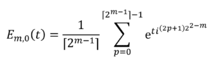
where
![]()
![]() (2.8)
(2.8)
Equation 2.7 and Equation 2.8 therefore show that ![]() can be written equivalently as a weighted sum of complex exponentials.
can be written equivalently as a weighted sum of complex exponentials.
The exponent ![]() can be decomposed using Euler’s formula. From
can be decomposed using Euler’s formula. From
![]() (2.9)
(2.9)
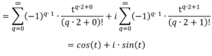
The special case ![]() gives us
gives us
![]() (2.10)
(2.10)
We can therefore write
![]() (2.11)
(2.11)
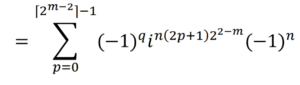
(2.12)![]()
(2.13)![]()
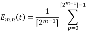
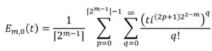
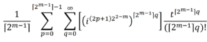
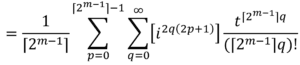
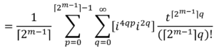
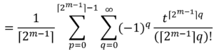
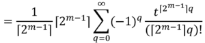
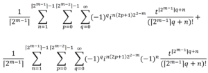
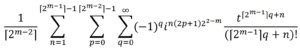
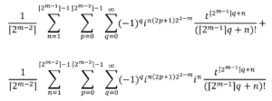
Equation 2.13 therefore allows us to rewrite Equation 2.8 as
![]()
![]() (2.14)
(2.14)
The first exponential factor,
![]() (2.15)
(2.15)
is a real-valued function that determines the rate of growth. The second exponential
factor,
![]() (2.16)
(2.16)
defines a circle in the complex plane with frequency
![]() (2.17)
(2.17)
The frequency information of ![]() (and, consequently, of
(and, consequently, of ![]() ) is therefore determined entirely by
) is therefore determined entirely by ![]() .
.
The key point is that ![]() is bounded from above: it cannot be higher than when
is bounded from above: it cannot be higher than when ![]() . This equality holds only for m = 2 (which, as shown in Appendix- A, corresponds to the standard Euler’s formula and generates the cosine and sine functions). Given m = 2, the possible values of p are 0 and 1, in either of which cases|
. This equality holds only for m = 2 (which, as shown in Appendix- A, corresponds to the standard Euler’s formula and generates the cosine and sine functions). Given m = 2, the possible values of p are 0 and 1, in either of which cases| ![]() | = 1. For any other m, we have
| = 1. For any other m, we have
![]() (2.18)
(2.18)
Therefore, if
![]() (2.19)
(2.19)
then all frequency information in ![]() will be contained within the bandwidth W.
will be contained within the bandwidth W.
Arranging for Equation 2.19 to hold is simply a matter of parameterizing correctly,
in terms of Equation 2.1. This is sufficient to complete the proof of Theorem 1, that ![]()
is not inherently constrained by the available bandwidth W.
However, restricting W is not without consequence. A smaller value of W increases 1/W and therefore the maximum value of t. If we look at Equation 2.14, this means that the growth factor, ![]() , reaches an exponentially higher value as W is decreased linearly. While the peak amplitude achieved is merely a choice of units, the shape of the amplitude growth curve is not altered by scaling. The implication is that decreasing W for constant has the effect of increasing the steepness of the exponential curves necessary to construct
, reaches an exponentially higher value as W is decreased linearly. While the peak amplitude achieved is merely a choice of units, the shape of the amplitude growth curve is not altered by scaling. The implication is that decreasing W for constant has the effect of increasing the steepness of the exponential curves necessary to construct ![]() , and therefore the slew rate (maximum rate of amplitude change) that the communication system must be able to support.
, and therefore the slew rate (maximum rate of amplitude change) that the communication system must be able to support.
An informal way of thinking about non-periodic channels is that information can be
conveyed through frequency-based or exponential-based parameters, or any combination. Decreasing the available bandwidth W has the effect of forcing information to be conveyed by increasingly rapid amplitude change in the available
frequency components.
Conversely, if we restrict the allowable growth in frequency components, then
increasing information capacity requires increasing the available bandwidth. In the limit of periodic channels, where frequency components are allowed only constant
amplitude, Shannon showed that we arrive at the information capacity formula
![]() (2.20)
(2.20)
This tells us that for a particular Signal-to-Noise Ratio (SNR), increasing the capacity
of a periodic channel requires a proportional increase in the available bandwidth.
It is interesting to see how the periodic limit arises from Equation 2.14. If we are
only allowed frequency components with constant amplitude, then we must build ![]() using only components
using only components![]() for which
for which
![]() (2.21)
(2.21)
This occurs only when m = 2. At m = 2, it is shown in Appendix A that precisely two functions ![]() are possible:
are possible: ![]() = cos(t) and
= cos(t) and ![]() = sin(t) . Hence,
= sin(t) . Hence, ![]() is fully specified by determining two coefficients, one each for
is fully specified by determining two coefficients, one each for ![]() and
and ![]() .
.
Since two coefficients are specified by two points, sampling twice in the period ![]() is sufficient to construct
is sufficient to construct ![]() . This establishes the Nyquist rate (Equation 2.3) as the limiting case for periodic channels.
. This establishes the Nyquist rate (Equation 2.3) as the limiting case for periodic channels.
We have seen that for non-periodic channels, the frequency of definition ![]() is not inherently limited by the available bandwidth W .
is not inherently limited by the available bandwidth W . ![]() is instead determined by available bandwidth and the maximum achievable slew rate. Slew rate plays a limiting role for exponential-based information transmission that is similar to the role that bandwidth plays for frequency-based information transmission.
is instead determined by available bandwidth and the maximum achievable slew rate. Slew rate plays a limiting role for exponential-based information transmission that is similar to the role that bandwidth plays for frequency-based information transmission.
To investigate this further, let us introduce notation. By “sr” is meant the slew rate observed in a particular communication system configuration; by “![]() ” is meant the slew rate observed when the communication system operates at the Nyquist rate (
” is meant the slew rate observed when the communication system operates at the Nyquist rate (![]() =
=![]() ) for a particular amount of available bandwidth ; by “
) for a particular amount of available bandwidth ; by “![]() ” is meant the maximum slew rate the communication system is capable of supporting.
” is meant the maximum slew rate the communication system is capable of supporting.
To understand the relationship between ![]() and slew rate, suppose that we wish to increase
and slew rate, suppose that we wish to increase ![]() without altering W. If signal power is also held constant, then the independence of the sample points requires that the statistical properties of the sample amplitudes cannot change; in particular, the maximum amplitude change between adjacent samples must remain the same when
without altering W. If signal power is also held constant, then the independence of the sample points requires that the statistical properties of the sample amplitudes cannot change; in particular, the maximum amplitude change between adjacent samples must remain the same when ![]() is increased. Since the time between samples decreases by the same amount that
is increased. Since the time between samples decreases by the same amount that ![]() increases, this means
increases, this means
that sr is proportional to ![]() .
.
Since ![]() cannot be increased beyond the point at which
cannot be increased beyond the point at which ![]() is reached without
is reached without
system failure, the extent to which ![]() can be increased beyond
can be increased beyond ![]() is proportional to
is proportional to
how much “extra” slew rate capacity is available at the Nyquist rate. More formally,
![]() (2.22)
(2.22)
This concludes our discussion of the frequency of definition, which determines the
sampling rate. The next section studies the use of sample amplitude information to
distinguish signals.
3. Power and Signal Distance
Let us assume that a non-periodic channel has been constructed to support a particular value of ![]() . The next thing we need to know is how distinct we can make
. The next thing we need to know is how distinct we can make
signals in terms of their amplitude sequences, subject to power constraints.
Following Shannon, we can think of a sequence of signal samples as ![]() defining coordinates in a space whose dimension is the total number of samples. Let be the length of the corresponding vector:
defining coordinates in a space whose dimension is the total number of samples. Let be the length of the corresponding vector:
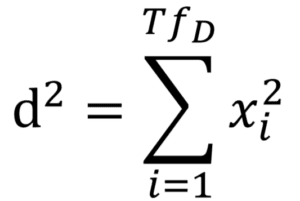 (3.1)
(3.1)
Where T is the time duration of the signal, and T![]() is therefore the total number of
is therefore the total number of
samples.
The larger d becomes, the easier it is to create noise-resistant separation between
different signals, and thereby increase the channel capacity. But since a larger requires more power, we would like to express d in terms of the power cost to achieve a given distance.
Shannon established the relationship
d² = 2WTP (3.2)
With P being the average (RMS) signal power.
However, his proof again implicitly assumes the channel is periodic.
It is possible to generalize Equation 3.2 for non-periodic channels as follows. The
energy transmitted by a wave is proportional to the square of its amplitude integrated over its duration. If ![]() is sufficiently high, we can approximate the energy
is sufficiently high, we can approximate the energy
integral with discrete amplitude boxes of duration 1/![]() each. Letting be the total wave energy, this gives us
each. Letting be the total wave energy, this gives us
![]() (3.3)
(3.3)
Which tells us that
![]() vv (3.4)
vv (3.4)
If we are limited to an average power budget P, then we can use E = TP to write Equation 3.4 as
![]() (3.5)
(3.5)
for non-periodic channels.
Notice that in the periodic limit, we have
![]() (3.6)
(3.6)
in which case the non-periodic distance formula (Equation 3.5) reduces to Shannon’s periodic distance formula (Equation 3.2).
4. Non-Periodic Channel Capacity
In the previous sections, we generalized the Nyquist rate and the signal distance
formula for non-periodic channels. In both cases, the necessary change was to
replace the Nyquist rate,![]() , with the frequency of definition,
, with the frequency of definition,![]() .
.
Given these two alterations, there are no further periodic assumptions in Shannon’s
proof. It can be generalized for non-periodic channels simply by replacing 2W by ![]()
throughout.
In Shannon’s notation, the channel capacity for a non-periodic channel is therefore
![]() (4.1)
(4.1)
This tells us that channel capacity increases linearly with the frequency of definition ![]() .
.
Using Equation 2.22 for the limiting value of ![]() , the above becomes
, the above becomes
![]() (4.2)
(4.2)
From the Nyquist rate (Equation 2.3) we can remove ![]() :
:
![]() (4.3)
(4.3)
Since Shannon’s original paper, it has become standard to represent the signal
power by S, rather than P, the bandwidth by B, rather than W, and to divide through
the ratio. In modern notation, therefore, the channel capacity for a non-periodic channel is given by
![]() (4.4)
(4.4)
Notice that in the periodic limit we replace ![]() with
with ![]() , rather than with
, rather than with ![]()
![]() ; this
; this
leads to the well-known periodic form of Shannon’s law:
![]() (4.5)
(4.5)
Comparing non-periodic channel capacity (Equation 4.4) to its periodic limit (Equation 4.5), the difference is of course the extra factor of ![]() for non-periodic channels.
for non-periodic channels.
This tells us that the relative advantage of a non-periodic channel over a periodic
channel is limited by its ability to handle high slew rates; or, more generally, by its
effective use of exponential information.
5. Conclusion
The current limitation of communication practice and theory to periodic channels is
something like painting with only half a palette. Frequency-based information has a
natural pairing with exponential-based information; combining the two increases
channel capacity and allows more options in system design.
It was shown in this report that the limiting role played by bandwidth for frequency-based information is played by slew rate for exponential-based information. The two together determine non-periodic channel capacity. For non-periodic channels, spectral efficiency can be increased beyond the periodic Shannon limit by effective use of exponential information.
Appendix A: Introduction to Cairns Space
This appendix provides a concise introduction to Cairns space, the mathematics used
in the proof of the generalized Shannon’s law for non-periodic channels.
The familiar Euler’s formula
![]() (A1)
(A1)
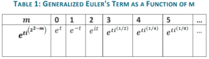
can be generalized by raising the imaginary constant on the left side to fractional powers. The new term
![]() (A2)
(A2)
reduces to Euler’s term in the special case m = 2 .
We can build the following table:
The standard Euler’s formula can be proved by expanding ![]() as a Taylor series and
as a Taylor series and
grouping real and imaginary terms. As shown in Appendix B, the same procedure can
also be used for fractional powers of i, starting from A2, to derive a generalization of
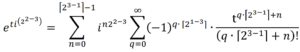
Euler’s formula for integer ![]() :
:
 (A3)
(A3)
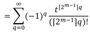
Where
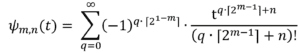 (A4)
(A4)
The ![]() may be called the “Cairns series functions”.
may be called the “Cairns series functions”.
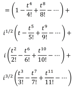
Notice that ![]() and
and ![]() give us the Taylor series for the standard cosine and
give us the Taylor series for the standard cosine and
sine functions, respectively.
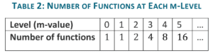
Each value of m produces a “level” of functions ![]() ; from the summation limits in Equation A3, each level has a total of
; from the summation limits in Equation A3, each level has a total of ![]() functions. That is:
functions. That is:
An important property of the ![]() is the regular pattern of their coefficients, as
is the regular pattern of their coefficients, as
shown in the below table.
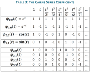
Here, the rows indicate the Taylor series coefficients for each ![]() . For instance, the row for
. For instance, the row for ![]() = cos(t) tells us that
= cos(t) tells us that
![]() (A5)
(A5)
From Table 3 it is easy to see, and not difficult to prove, that the ![]() coefficients define a set of orthogonal vectors. More precisely, if M is a positive integer, then the vectors formed from the first
coefficients define a set of orthogonal vectors. More precisely, if M is a positive integer, then the vectors formed from the first ![]() coefficients of the functions
coefficients of the functions ![]() for 0 ≤ m ≤ M constitute a set of orthogonal basis vectors for a
for 0 ≤ m ≤ M constitute a set of orthogonal basis vectors for a ![]() -dimensional space. These can be normalized to produce the orthonormal “
-dimensional space. These can be normalized to produce the orthonormal “![]() Cairns basis vectors”.
Cairns basis vectors”.
The existence of the ![]() Cairns basis vectors implies that any Taylor polynomial P of
Cairns basis vectors implies that any Taylor polynomial P of
degree k<![]() can be orthogonally projected onto polynomials formed from the first
can be orthogonally projected onto polynomials formed from the first ![]() terms of the Cairns series functions simply by taking the inner product of P’s coefficients with the
terms of the Cairns series functions simply by taking the inner product of P’s coefficients with the ![]() Cairns basis vectors.
Cairns basis vectors.
The first ![]() terms of the Cairns series functions
terms of the Cairns series functions ![]() are only an approximation to the full infinite series expansion of the
are only an approximation to the full infinite series expansion of the ![]() . However, the error in the approximation is
. However, the error in the approximation is ![]() , with a reciprocal factorial coefficient, and therefore falls off very rapidly as M increases. For high-degree polynomials, therefore, it is reasonable to speak of projecting onto the
, with a reciprocal factorial coefficient, and therefore falls off very rapidly as M increases. For high-degree polynomials, therefore, it is reasonable to speak of projecting onto the ![]() by this procedure
by this procedure
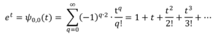
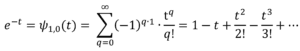
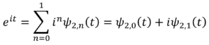
It is well-known that the cosine and sine functions of Euler’s formula can be represented not only by Taylor series but also by sums of complex exponentials.
Explicitly:
![]() (A6)
(A6)
and
![]() (A7)
(A7)
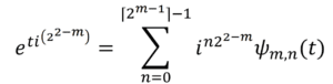
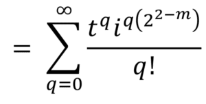
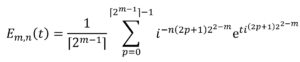
This characteristic also holds for the generalized Euler’s formula. We can define
 (A8)
(A8)
Where the![]() may be called the “Cairns exponential functions.”
may be called the “Cairns exponential functions.”
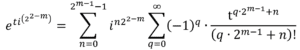
By expanding the right side of Equation A8 as a sum of Taylor polynomials and
recursively cancelling terms, it is shown in Appendix C that for all m and n
![]() (A9)
(A9)
Equation A9 tells us that once a polynomial has been projected onto the Cairns series functions, it can be immediately converted into a sum of complex exponentials.
Appendix B: The Generalized Euler’s Formula Expressed as Series Functions
In Appendix A, it was stated that for integer m ≥ 0
![]() (B1)
(B1)
Where
 (B2)
(B2)
This appendix proves that assertion.
Three special cases of this identity are well-known, as shown below.
For m = 0, Equation B1 becomes
 (B3)
(B3)
For m = 1 , Equation B1 becomes
 (B4)
(B4)
For m = 2 , Equation B1 becomes
 (B5)
(B5)
=
The general case of Equation B1 can be proved by expanding ![]() as a Taylor polynomial and grouping terms. This proceeds as follows.
as a Taylor polynomial and grouping terms. This proceeds as follows.
 (B6)
(B6)
Notice that when
![]() (B7)
(B7)
we have
![]() (B8)
(B8)
This tells us that every ![]() steps the pattern of
steps the pattern of ![]() will repeat, with alternating sign. Let us call
will repeat, with alternating sign. Let us call ![]() the “step size”. Since we are interested in grouping terms with like powers of i, we want to separate the series into subseries with terms separated by the step size. This gives us (roughly)
the “step size”. Since we are interested in grouping terms with like powers of i, we want to separate the series into subseries with terms separated by the step size. This gives us (roughly)
 (B9)
(B9)
This is correct except for the case m = 0 , which corresponds to ![]() . We have two problems for m = 0: these are that
. We have two problems for m = 0: these are that![]() = 1/2 (we would like it to equal 1 ); and that the sign should not alternate for
= 1/2 (we would like it to equal 1 ); and that the sign should not alternate for ![]() .
.
These problems can be fixed by adjusting Equation B9 as follows:
 (B10)
(B10)
If we label the second summation ![]() then we have Equation B1 and Equation
then we have Equation B1 and Equation
B2.
We have seen that Equation B10 (or, equivalently, Equation B1 and Equation B2) reduce to familiar cases for m = 0, m = 1, and m = 2. As an example of an unfamiliar case, consider m = 3. We then have
 (B11)
(B11)
Which simplifies to
 (B12)
(B12)
Appendix C: The Equivalence of the Cairns Series and Exponential Functions
In Appendix A, it was stated that
![]() (C1)
(C1)
Where
 (C2)
(C2)
and
 (C3)
(C3)
This appendix proves that assertion.
Four special cases of this identity are well-known, as shown below.
For m = 0, n = 0, Equation C1 becomes
![]() (C4)
(C4)
For m = 1, n = 0 , Equation C1 becomes
![]() (C5)
(C5)
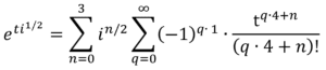
For m = 2, n = 0, , Equation C1 becomes
![]() (C6)
(C6)
For m = 2, n = 1, Equation C1 becomes
![]() (C7)
(C7)
It may be seen by inspection of Equation C2 that ![]() is the integral of
is the integral of ![]() , with constant of integration zero. This is similarly true for
, with constant of integration zero. This is similarly true for ![]() , as can be seen either directly from Equation C3 or by examining the polynomial sequences expanded in Appendix B.
, as can be seen either directly from Equation C3 or by examining the polynomial sequences expanded in Appendix B.
Therefore, to prove Equation C1 it is sufficient to prove the case for n = 0:
![]() (C8)
(C8)
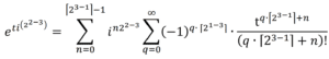
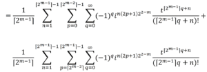
as equality for all other values of n will follow from parallel integration. The proof of Equation C8 follows from expanding ![]() as a sum of Taylor series and recursively canceling terms. This proceeds as follows.
as a sum of Taylor series and recursively canceling terms. This proceeds as follows.
 (C9)
(C9)
 (C10)
(C10)
Using an idea similar to Appendix B, we break the summation into subseries in which the terms are separated by a step size of ![]() . With the new index variable being n, this gives us
. With the new index variable being n, this gives us
![]() (C11)
(C11)
Now, separate out the imaginary factor:
![]() (C12)
(C12)
If we look at the case n = 0 by itself, the right side of Equation C12 becomes
 (C13)
(C13)
 (C14)
(C14)
 (C15)
(C15)
 (C16)
(C16)
 (C17)
(C17)
 (C18)
(C18)
![]() (C19)
(C19)
This shows that the n = 0 subseries of Equation C12 satisfies ![]() . The proof of Equation C1 therefore depends on the n > 0subseries of Equation C12 summing to precisely zero. We show that next.
. The proof of Equation C1 therefore depends on the n > 0subseries of Equation C12 summing to precisely zero. We show that next.
Removing the n = 0 subseries from Equation C12, we have
![]() (C20)
(C20)
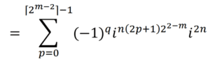
Next, we simplify the complex factor:
![]() (C21)
(C21)
![]() (C22)
(C22)
![]() (C23)
(C23)
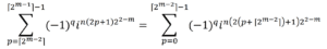
Now, split Equation C23 into two parts by dividing the p summation in half:
 (C24)
(C24)
We will now change the p parameterization of the second summation, so it can be
compared to the first.
 (C25)
(C25)
 (C26)
(C26)
 (C27)
(C27)
Update C24 with the re-parameterized second summation, using C27. This gives
 (C28)
(C28)
The two summations differ only by a factor of ![]() . This means that the
. This means that the
summations will cancel to zero for any odd n. So only even values of n > 0 could
potentially contribute a nonzero sum to Equation C12. We next show that values of n > 0 that are divisible by two sum to zero.
For even , the summations in C28 will be equal, so we can add them to produce
 (C29)
(C29)
We now repeat the procedure of splitting the p summation in two, then reparameterizing p for the second summation This gives us
 (C30)
(C30)
C28 showed that odd values of n sum to zero; C30 shows in addition that if n contains an odd number of factors of the summation will be zero.
This process can be repeated a total of m – 1 times to show that all values of n >0
sum to zero. This is sufficient to prove Equation C1.
1Shannon, C.E. (1949). Communication in the presence of noise. Proc. IRE, 37, 10-21
2For ease of comparison with Shannon’s proof, his notation is adopted as far as possible: in this case, the use of “W” for bandwidth.
3Prothero, J. (2007). Euler’s formula for fractional powers of i. Available from www.astrapi-corp.com