Jerrold Prothero, Ph.D.
[email protected]
April 15, 2007
Copyright c 2007 Jerrold Prothero. All rights reserved.
May be distributed freely in unaltered form
To Leonhard Euler, on the occasion of his 300th birthday.
Having lived, they live forever,
Who to purpose grand endeavor.
And nor shall time, nor tongue of man,
E’er taint or burnish that rare clan;
For none may mark them with their sign,
Who chose to breathe the breath divine.
Contents
1 Introduction
2 The Magic Suitcase
3 The Geometric Interpretation
4 The Taylor Series Interpretation
5 The Algebraic Interpretation
6 Projection Onto Cairns Space
7 The Broom Theorems 21
7.1 Sweeping Up
7.2 Sweeping Down
7.3 Sweeping Sideways
8 Sundry Findings
8.1 Pythagorean Identitie
8.2 Curvature
8.3 The Inner Product on Level m
8.4 Differentiation, Rotation and Displacement
8.5 The Roots of nth-Degree Polynomials
9 Conclusion
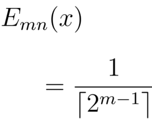
A Derivation of ψmn(x)
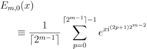
B Proof of the Equivalence of ψmn(x) and Emn(x)
C Factoring Emn(x)
C.1 Derivation of Em,0 Factors
C.2 Emn(x)
D The Orthogonality of ψmn(x) Coefficients
E Derivation of the Broom Theorems
E.1 Sweeping Up
E.2 Sweeping Sideways
F Derivation of the Inner Product
G The Cairns Functions For m ≤ 4
G.1 m ≤ 0
G.2 m = 1
G.3 m = 2
G.4 m = 3
G.5 m = 4
Abstract
A generalization of Euler’s formula ![]() for fractional powers
for fractional powers
of i is discussed. This generalization, based on the term
corresponds to a sequence of spirals in the complex plane. Just as ![]() generates cos(x) and sin(x),
generates cos(x) and sin(x), ![]() generates sets of functions (“levels”) which generalize the properties of cos(x) and sin(x) by combining periodic and exponential characteristics. The set of all functions generated by
generates sets of functions (“levels”) which generalize the properties of cos(x) and sin(x) by combining periodic and exponential characteristics. The set of all functions generated by ![]() defines an orthogonal basis for the set of all Taylor polynomials.
defines an orthogonal basis for the set of all Taylor polynomials.
Chapter 1
Introduction
Asclepius, in days when we are young,
The Music of the Spheres we first hear sung!
Through straining then, to listen and to learn,
What revelries of truth one may discern!
According to Richard Feynman, Euler’s formula¹
![]() (1.1)
(1.1)
is the most remarkable in mathematics.
Certainly, it is one of the most important, relating the exponential constant
e, which describes growth, to the cos(x) and sin(x) functions, which describe
periodic behavior, through the constant i, which describes rotations.
It is odd, given the importance of the equation, that there does not appear to
exist a systematic discussion of the implications of raising i in Euler’s formula to
fractional powers. As will be shown here, there is a natural extension of Euler’s
formula for fractional powers of i that provides coherent and interesting results.
Implications include
- While Euler’s formula corresponds to a circle in the complex plane, fractional powers of i correspond to spirals.
- By varying a single parameter, it is possible to generate
 , and an infinite family of related functions.
 - Just as generates cos(x) and sin(x), each fractional power of i considered here generates its own set of functions (a “level”). The levels have related but distinct properties.
- The set of functions at each level form a differential cycle. That is, every function in the cycle is the derivative of the next higher function in the
cycle, with the highest function being the negative derivative of the lowest. - Each generated function can be represented in terms of a combination of
hyperbolic and circular components. More precisely, every such function
is either or a sum of products of either cosh(x) or
sinh(x) with either cos(x) or sin(x). - The set of functions generated at all levels defines an orthogonal basis for
the Taylor polynomials - A geometric curvature can be associated with Taylor polynomials.
- In certain cases, the roots of nth–degree polynomials can be found very
simply.
I have attempted to make this monograph accessible to as wide an audience
as possible: mathematics should not be left solely to specialists. References to
background topics are collected online at http://del.icio.us/jprothero/Euler
See also jerroldprothero.blogspot.com
Chapter 2
The Magic Suitcase
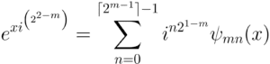
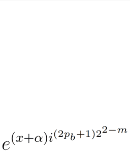
Of all fractions, perhaps the simplest are those which are powers of two ( ![]() etc.). Consequently, in considering possible generalizations of Euler’s term to fractional powers of i we are led naturally to the term
etc.). Consequently, in considering possible generalizations of Euler’s term to fractional powers of i we are led naturally to the term
 (2.1)
(2.1)
Where m is an integer. I call this the “magic suitcase”, because however much one unpacks from this term, there is always more to be found.
While perhaps initially mysterious, the suitcase simply takes advantage of the useful properties of powers of two, which interact very naturally with i. Each value of m corresponds to a particular level, whose characteristics are outlined below.
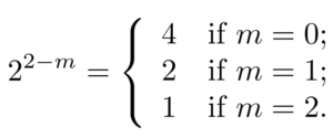
- For m = 0 (and, similarly, for any negative value of m) the i exponent
reduces to
so the suitcase is equal to the familiar natural exponential, - For m = 1, the suitcase reduces to
This gives us the traditional Euler term, corresponding to a circle in the
complex plane. - For m = 3, we have
which (as we will see) corresponds to a spiral in the complex plane. - For m = 4, we have corresponding to a (different) spiral in the
complex plane. - And so on. As m becomes very large, we have
so
The suitcase term both “starts” (m = 0) and “ends” (m → ∞) with ![]() . We will soon see a geometric interpretation of why this is true. The line of thought discussed here was originally inspired by the term
. We will soon see a geometric interpretation of why this is true. The line of thought discussed here was originally inspired by the term
![]() (2.2)
(2.2)
provided by John Cairns in U.S. Patent 5,563,556, Geometrically Modulated Waves. 1 Aside from a certain ungainliness, the Cairns term has technical limitations and the patent itself contains several algebraic errors.
Nonetheless, so far as I know (and, apparently, so far as the Patent Office knew), Cairns was the first to examine the consequences of fractional powers of i in Euler’s formula. Consequently, it is appropriate to refer to the set of functions described below as “Cairns space”.
Chapter 3
The Geometric
Interpretation
A well-known consequence of Euler’s formula is that ![]() 2 Therefore
2 Therefore
![]() (3.1)
(3.1)
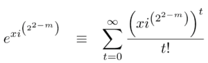
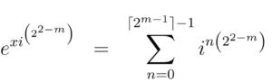
By replacing ![]() with
with ![]() in the suitcase, we can express it equivalently as
in the suitcase, we can express it equivalently as
![]() (3.2)
(3.2)
![]() (3.3)
(3.3)
![]() (3.4)
(3.4)
We can now invoke Euler’s formula to break apart the upper exponent:
![]() (3.5)
(3.5)
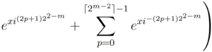
By plugging Equation (3.5) in for the exponent of Equation (3.4), we get
![]() (3.6)
(3.6)
![]() (3.7)
(3.7)
and therefore
![]() (3.8)
(3.8)
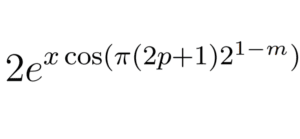
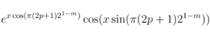
The first factor of Equation (3.8),![]() , is a pure real-valued exponential. The second factor,
, is a pure real-valued exponential. The second factor, ![]() is a pure real-valued exponential. The second factor,
is a pure real-valued exponential. The second factor, ![]() . Multiplying these two factors together, we have a “growing circle”: that is, a spiral
. Multiplying these two factors together, we have a “growing circle”: that is, a spiral
As m increases, we have
![]() (3.9)
(3.9)
![]() (3.10)
(3.10)
Consequently, with increasing m the exponential term grows faster, and the
spiral rotation “slows down” (period increases).
Regardless of the value of m, for x = 0 we have ![]() Therefore, every spiral “starts” on the real axis of the complex plane, at the point (1, 0). As m increases, the period also increases: in the limit of large m, the spiral “slows down” its rotation to the degree that it never gets off the real axis. This is the geometric interpretation of the fact that
Therefore, every spiral “starts” on the real axis of the complex plane, at the point (1, 0). As m increases, the period also increases: in the limit of large m, the spiral “slows down” its rotation to the degree that it never gets off the real axis. This is the geometric interpretation of the fact that ![]() converges back to
converges back to ![]() as m → ∞.
as m → ∞.
For clarity, let us look at Equation (3.8) for particular values of m.
- For m = 0 (and similarly for any negative value of m) 1 and so
- For m = 1, −1 and so
- For m = 2, 0 and , so
- For large m, so
These results are of course consistent with those found in Chapter 1.
Incidentally, by invoking the Euler formula and its equivalent for hyperbolic
trigonometry
![]() (3.11)
(3.11)
we can decompose Equation (3.8) into
![]()
![]() (3.12)
(3.12)
As we shall see, this balanced treatment of hyperbolic and circular functions
is intrinsic to Cairns space.
Chapter 4
The Taylor Series
Interpretation
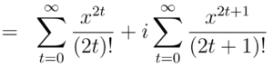
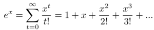
It is well-known that Euler’s formula can be derived by expanding ![]() as a Taylor series and grouping terms. One gets
as a Taylor series and grouping terms. One gets
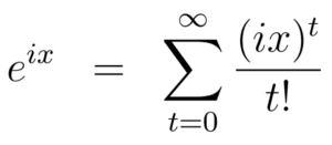 (4.1)
(4.1)
![]() (4.2)
(4.2)
![]() (4.3)
(4.3)
![]() (4.4)
(4.4)
 (4.5)
(4.5)
![]() (4.6)
(4.6)
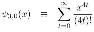
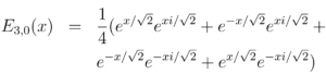
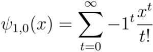
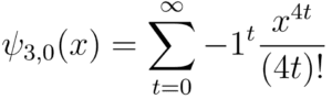
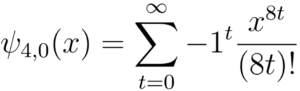
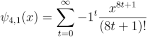
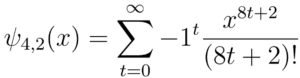
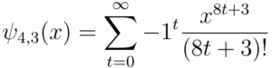
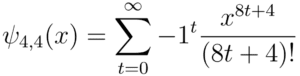
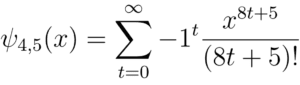
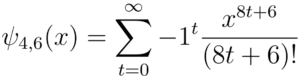
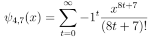
Precisely the same procedure can be followed to generate functions for any
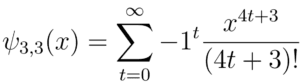
m-value of the suitcase. For m = 3, we have
![]() (4.7)
(4.7)
![]() (4.8)
(4.8)
![]() (4.9)
(4.9)
![]()
![]() (4.11)
(4.11)
![]() (4.12)
(4.12)
![]() (4.13)
(4.13)
= ![]() (4.14)
(4.14)
Where
 (4.15)
![]() (4.16)
(4.16)
![]() (4.17)
(4.17)
![]() (4.18)
(4.18)
(4.19)
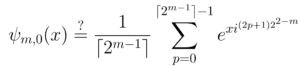
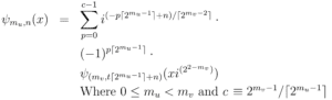
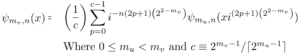
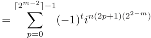
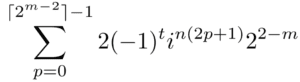
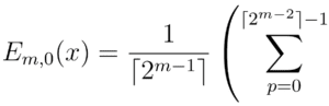
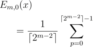
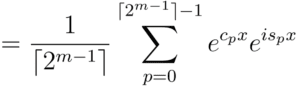
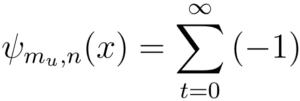
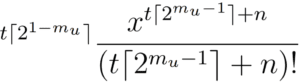
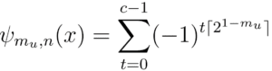
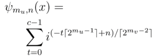
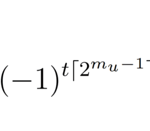
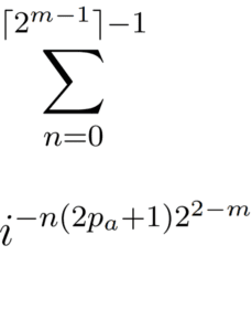
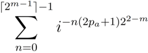
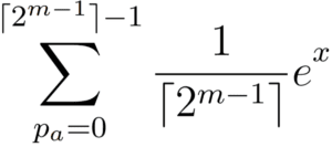
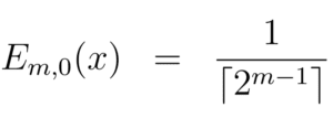
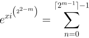
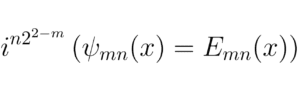
The general relationship for any m is 3
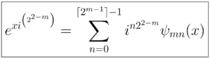 (4.20)
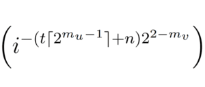
where
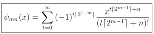 (4.21)
The ceiling functions are there to handle boundary cases correctly. The
ceiling function prevents ![]() from taking on a fractional value for m ≤ 0. In
from taking on a fractional value for m ≤ 0. In
Equation (4.21) the factor ![]() “turns off” the sign alternation of terms for
“turns off” the sign alternation of terms for
m ≤ 0, corresponding the function ![]() .
.
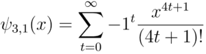
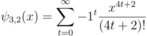
Here are some interesting points about Equations (4.20) and (4.21).
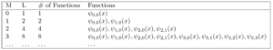
- The value of m determines a “level” of Cairns space, defining a set of
functions.– m < 0 corresponds to the single function
– m = 1 corresponds to the single function
– m = 2 corresponds to the two functions and
– m = 3 corresponds to the four functions and as defined above
– m = 4 corresponds to eight functions
– In general, for any m there are functions. - The value of n determines a particular function at level m. The possible
values of n run from 0 to − 1. - • At level m, the Taylor series corresponding to consist of terms
with powers differing by −1 e and offset by n. - If n is even, all terms in have even power; if n is odd, all terms in have odd power. Consequently, is symmetric for even n and anti-symmetric for odd n. 4
- For m > 1, we see by inspection that the functions in level m form a differential cycle. That is, for and for n = 0 we have
Chapter 5
The Algebraic
Interpretation
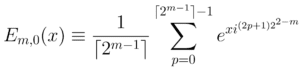
In Chapter 4, we saw how to express the functions generated by ![]() as Taylor series. Is it also possible to describe these same functions in terms of familiar algebraic expressions? In this chapter, we shall see that it is.
as Taylor series. Is it also possible to describe these same functions in terms of familiar algebraic expressions? In this chapter, we shall see that it is.
From Chapter 4 we know that
![]() (5.1)
(5.1)
![]() (5.2)
(5.2)
![]() (5.3)
(5.3)
Note that
 (5.4)
(5.4)
So the above equations all have ![]() as the first term. Notice also that the above three equations can be described by the rules.
as the first term. Notice also that the above three equations can be described by the rules.
- Start with the term
- If (1 + 2) < 4, add the term
- Divide by the number of terms
This might lead one to guess 5 that
![]() (5.5)
(5.5)
![]() (5.6)
(5.6)
![]() (5.7)
(5.7)
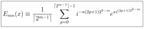
and that in general 6
 (5.8)
(5.8)
To prove Equation (5.8), it is useful to define a function ![]() with the above property. By definition
with the above property. By definition
 (5.9)
(5.9)
If we assume ![]() , it follows that the derivative and integrals of
, it follows that the derivative and integrals of ![]() must be equal to the derivatives and integrals of
must be equal to the derivatives and integrals of ![]() . By inspection, taking the integrals of Equation (5.9) with integration constant zero, we define
. By inspection, taking the integrals of Equation (5.9) with integration constant zero, we define
 (5.10)
With the above definition of ![]() we can then prove that for all m,
we can then prove that for all m,
![]() (5.11)
(5.11)
as is shown in Appendix B.7
The equivalence of ![]() and
and ![]() is quite interesting, as it relates
is quite interesting, as it relates
an infinite set of Taylor series to a corresponding infinite set of exponential functions. One has two different ways of looking at the component functions of ![]()
Because ![]() =
= ![]() , by comparison with Equation (4.20) we must
, by comparison with Equation (4.20) we must
have
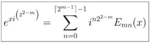 (5.12)
Since ![]() is always a real-valued function, it follows that
is always a real-valued function, it follows that ![]() must also be always real-valued. This is rather surprising, given that for n 6= 0 the terms of
must also be always real-valued. This is rather surprising, given that for n 6= 0 the terms of ![]() have imaginary coefficients. With each successive differentiation of
have imaginary coefficients. With each successive differentiation of ![]() a shower of imaginary factors descend from the exponents to become coefficients; and yet the imaginary part of
a shower of imaginary factors descend from the exponents to become coefficients; and yet the imaginary part of ![]() always exactly cancels out to produce a purely real result. It is a most delicate dance.
always exactly cancels out to produce a purely real result. It is a most delicate dance.
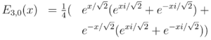
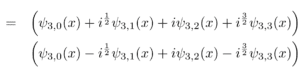
Let us examine ![]() in more detail. For m = 3, we have
in more detail. For m = 3, we have
![]() (5.13)
(5.13)
We can use the method of Chapter 3 to write
![]() (5.14)
(5.14)
![]() (5.15)
(5.15)
![]() (5.16)
(5.16)
![]() (5.17)
(5.17)
![]() (5.18)
(5.18)
![]() (5.19)
(5.19)
![]() (5.20)
(5.20)
 (5.21)
![]() (5.22)
(5.22)
![]() (5.23)
(5.23)
 (5.24)
 (5.25)
![]() (5.26)
(5.26)
![]() (5.27)
(5.27)
![]() (5.28)
(5.28)
![]() (5.29)
(5.29)
And hence
 (5.30)
We can now factor Equation (5.30) by combining like factors to obtain
 (5.31)
![]() (5.32)
(5.32)
![]() (5.33)
(5.33)
Following the differentiation rule for ![]() given in Chapter 4, we obtain
given in Chapter 4, we obtain
![]() (5.34)
(5.34)
![]() (5.35)
(5.35)
![]() (5.36)
(5.36)
![]() (5.37)
(5.37)
(5.38)
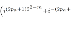
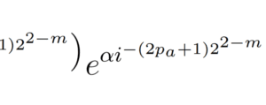
As shown in Appendix C, for m ≥ 2 the general rule is
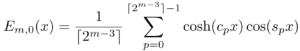 (5.39)
Where we have used the short-hands
![]() (5.40)
(5.40)
![]() (5.41)
(5.41)
From ![]() , we can obtain
, we can obtain ![]() for all n by repeated differentiation
for all n by repeated differentiation
or integration. Alternatively, one can find ![]() from the following equation
from the following equation
(see Appendix C)
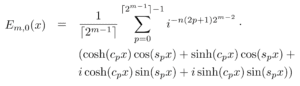 (5.42)
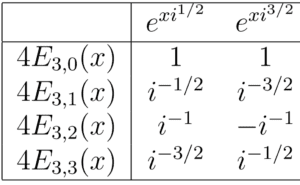
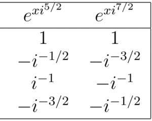
For concreteness, the algebraic view of the Cairns functions for m ≤ 4 are
given in Appendix G.
Recall from Chapter 4 that ψmn(x) is symmetric if n is even, and antisymmetric if n is odd. The same rule must hold for ![]() , since
, since ![]() =
= ![]() . From the
. From the ![]() perspective, the symmetry rules hold because cosh(x) and cos(x) are symmetric functions, and sinh(x) and sin(x) are antisymmetric. The product of two symmetric functions or two anti-symmetric functions is symmetric, and the product of a symmetric with an anti-symmetric function is anti-symmetric. For even n,
perspective, the symmetry rules hold because cosh(x) and cos(x) are symmetric functions, and sinh(x) and sin(x) are antisymmetric. The product of two symmetric functions or two anti-symmetric functions is symmetric, and the product of a symmetric with an anti-symmetric function is anti-symmetric. For even n, ![]() is a sum of products of the (symmetric) cosh(x) cos(x) and sinh(x) sin(x); for odd n,
is a sum of products of the (symmetric) cosh(x) cos(x) and sinh(x) sin(x); for odd n, ![]() is a sum of products of the (anti-symmetric) cosh(x) sin(x) and sinh(x) cos(x).
is a sum of products of the (anti-symmetric) cosh(x) sin(x) and sinh(x) cos(x).
Chapter 6
Projection Onto Cairns
Space
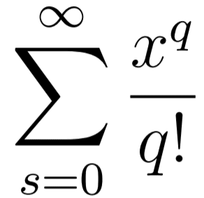
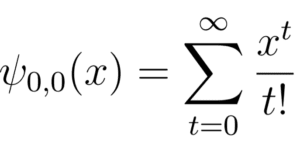
The simplest of all infinite Taylor series is
 (6.1)
(6.1)
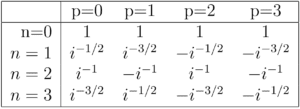
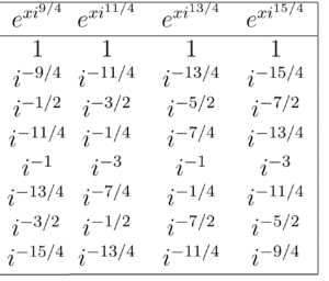
By inspection of Equation (4.21), we see that every ![]() can be derived from the Taylor series for
can be derived from the Taylor series for ![]() by taking the terms of
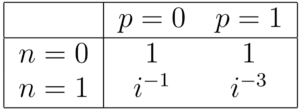
by taking the terms of ![]() and multiplying each of them by either −1, 0, or 1. More explicitly, we can build the below table, in which each entry gives the coefficient of a particular
and multiplying each of them by either −1, 0, or 1. More explicitly, we can build the below table, in which each entry gives the coefficient of a particular ![]() for a particular term in
for a particular term in ![]() .
.
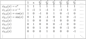
On examining this table, one is struck by a very regular pattern. If we interpret the entries in each row as components of a vector in Euclidean space, it is fairly evident that the vectors are orthogonal.
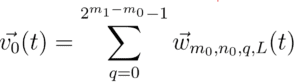
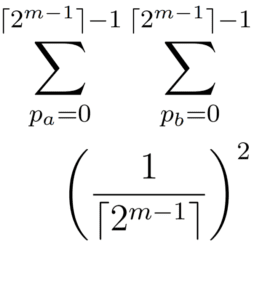
To formalize this idea, let us define the vectors corresponding to the above
table as follows. We take a finite approximation to Cairns space, where we consider only the first M levels and the first ![]() terms from functions in each of these levels. We recover the full Cairns space in the limit as M → ∞.
terms from functions in each of these levels. We recover the full Cairns space in the limit as M → ∞.
![]() (6.2)
(6.2)
for
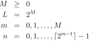
M ≥ 0 (6.3)
L = ![]() (6.4)
(6.4)
m ≥ 0, 1, . . . , M (6.5)
n ≥ 0, 1, . . . , ![]() – 1 (6.6)
– 1 (6.6)
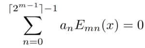
As is proved in Appendix D, this set of vectors is orthogonal: i.e.,
![]() Unless
Unless ![]() (6.7)
(6.7)
Notice that L is equal to the total number of Cairns functions through level
M. More explicitly,
This is a quite useful feature. It tells us that the first L vectors as defined above form an orthogonal set covering all Taylor series with degree less than L. Consequently, any Taylor polynomial can be reversibly projected onto (a finite approximation of) Cairns space simply by computing a series of L dot products. And since the vectors to be projected onto contain only −1, 0 and 1 entries, computing the dot products requires only addition and subtraction of the terms in the Taylor series, followed by a divide to scale for the length of the vector projected onto.
We can normalize the vectors defined above into an orthonormal basis set by dividing each by its length. Since the fraction of terms that are non-zero at level m is ![]() , the number of non-zero terms in
, the number of non-zero terms in ![]() is
is ![]() . Since the non- zero terms are all either 1 or −1, the vector length is
. Since the non- zero terms are all either 1 or −1, the vector length is
![]() (6.8)
(6.8)
and of course the normalized basis vectors are
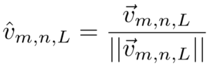 (6.9)
(6.9)
In this chapter, we have seen that any function defined by a Taylor series
can be trivially and reversibly mapped onto the Cairns functions by orthogonal
projection. Once this mapping is complete, the function can be viewed in terms
of its hyperbolic and circular components, simply by switching to the algebraic
(![]() ) interpretation.
) interpretation.
Doing so provides a decomposition similar to Fourier analysis; but while
Fourier analysis represents only the periodic properties of the source function,
Cairns space provides a balanced treatment of both exponential and periodic
characteristics.
It may also be of interest that after projecting onto Cairns space one can measure a curvature associated with a function, in the sense outlined in Section 8.2, by calculating the relative weight of the projection on higher m-levels.
Chapter 7
The Broom Theorems
While the ![]() functions define linearly-independent vectors, in the sense described in Chapter 6, there are methods to move between them using nonlinear ransforms. I call the methods for doing so the “broom theorems”, since they allow information to be “swept” to different parts of Cairns space. To sweep up or down through the levels of Cairns space requires imaginary factors. It is also possible to “sweep sideways” at a particular level, through use of a displacement.
functions define linearly-independent vectors, in the sense described in Chapter 6, there are methods to move between them using nonlinear ransforms. I call the methods for doing so the “broom theorems”, since they allow information to be “swept” to different parts of Cairns space. To sweep up or down through the levels of Cairns space requires imaginary factors. It is also possible to “sweep sideways” at a particular level, through use of a displacement.
Roughly speaking,
- To sweep from a lower level mu to a higher level , we pick a set of that cover the same terms as a given , use an imaginary factor to “turn off” the sign alternation at level mv, then pick the appropriate sign for each function at level mv to build up the .
- To sweep from a higher level to a lower level mu, we pick the function at level mu that covers the same terms. It will also cover other terms. We duplicate the function at level and use imaginary factors to cancel out
the terms we do not need. - • To move sideways at a given m-level, we expand a function in its Taylor
series, then group it in terms of the other functions at the same level in
such a way that the original function is spread over all functions at that
level.
The formalizations are provided below. See Appendix E for proofs.
7.1 Sweeping Up
To move from a lower to a higher m-level, we have
 (7.1)
(7.1)
Here are examples, which can be checked by expanding their Taylor series.
- Map to level m = 1. = 0, mv = 1, n = 0, c = 1. We have , which is equivalent to the statement that .
- Map to level m = 2. = 0, = 2, n = 0, c = 2. We have , which is equivalent to the statement . This is in a sense the inverse of Euler’s formula; it is also equivalent to the hyperbolic identity .
- Map = to level m = 2. = 1, = 3, v = 2, n = 0, c = 2. We have , which is equivalent to the statement .
- Map x to level m = 3. . We
have. - Map to level m = 4. = 2, = 4, n = 1, c = 4. We
have
![]()
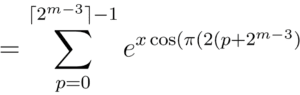
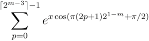
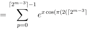
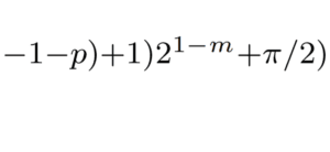
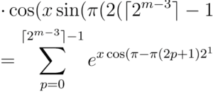
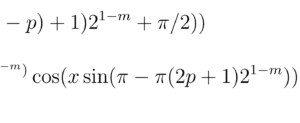
7.2 Sweeping Down
 (7.2)
(7.2)
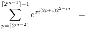
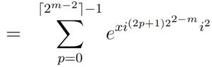
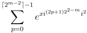
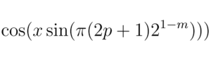
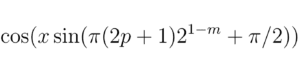
The ![]() factor in the
factor in the ![]() argument is designed to provide a sign alternation every
argument is designed to provide a sign alternation every ![]() terms, which corresponds to the sign alternation pattern
terms, which corresponds to the sign alternation pattern
for level mv. The (2p + 1) factor is designed to cancel out the unwanted terms at level![]() . The coefficient of
. The coefficient of ![]() performs a shift to handle n > 0
performs a shift to handle n > 0
correctly.
Notice that in the special case ![]() = 0, Equation (7.2) reduces to Equation (5.10). From this viewpoint, Equation (5.10) is simply the special case where one sweeps down to level m = 0. The proof of Equation (7.2) is therefore similar to the proof of Equation (5.10), differing in the number of stages required.
= 0, Equation (7.2) reduces to Equation (5.10). From this viewpoint, Equation (5.10) is simply the special case where one sweeps down to level m = 0. The proof of Equation (7.2) is therefore similar to the proof of Equation (5.10), differing in the number of stages required.
Here are some examples
- Map . We have which is equivalent to the statement that .
- Map . We have which is equivalent to the statement
that, familiar from trigonometry. - Map ψ2,0(x) = cos(x) to ψ0,0(x). = 2, = 0, n = 0, c = 2. We have , which is equivalent to the statement that , equivalent to the above.
- Map ψ3,0(x) to ψ2,0(x). = 3, = 2, n = 0, c = 2. We have, which can be checked by expanding the corresponding Taylor series.
- .Map ψ3,0(x) to ψ0,0(x). = 3, = 0, n = 0, c = 4. We have
ψ3,0 = , which again can
be checked by expanding the Taylor series. - Map ψ3,1(x) to ψ2,1(x). = 3, = 2, n = 1, c = 2. We have , again checkable from the Taylor series.
7.3 Sweeping Sideways
We can spread any function at level m over all of the functions at level m by
introducing a displacement. The general rule is as follows (see Appendix E for
a proof)
![]()
(7.3)
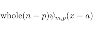
Where we define whole(n − p) = 1 for (n − p) ≥ 0 and −1 other 8
For instance
- For m = 0, n = 0, we have ψ0,0(x) = ψ0,0(x − a)ψ0,0(a), which in more
familiar notation reads. - For m = 2, n = 0 we have ψ2,0(x) = ψ2,0(x−a)ψ2,0(a)−ψ2,1(x−a)ψ2,1(a), or equivalently cos(x) = cos(x − a) cos(a) − sin(x − a) sin(a). With the change of variables u = x − a, v = a, this is equivalent to the familiar double-angle formula cos(u + v) = cos(u) cos(v) − sin(u) sin(v).
- For m = 2, n = 1 we have ψ2,1(x) = ψ2,0(x−a)ψ2,1(a)+ψ2,1(x−a)ψ2,0(a),
or equivalently sin(x) = cos(x − a) sin(a) + sin(x − a) cos(a), which again
is a familiar double-angle formula. - For m = 2, n = 1 we have ψ2,1(x) = ψ2,0(x−a)ψ2,1(a)+ψ2,1(x−a)ψ2,0(a),
or equivalently sin(x) = cos(x − a) sin(a) + sin(x − a) cos(a), which again
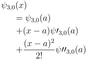
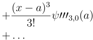
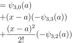
is a familiar double-angle formula. - For m = 3, n = 0 we have
ψ3,0(x) = ψ3,0(x−a)ψ3,0(a)−ψ3,1(x−a)ψ3,3(a)−ψ3,2(x−a)ψ3,2(a)−ψ3,3(x−a)ψ3,1(a)
Chapter 8
Sundry Findings
This chapter collects findings that are either not sufficiently important, or not
sufficiently developed, to merit their own chapters.
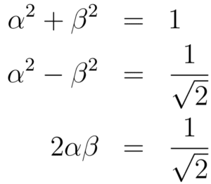
8.1 Pythagorean Identities
Consider the well-known identity cos²(x) + sin²(x) = 1. This can be derived from Euler’s formula by comparing
![]() (8.1)
(8.1)
![]()
![]() (8.2)
(8.2)
= (cos(x) + i sin(x))(cos(x) − i sin(x)) (8.3)
= cos(x) cos(x) + sin(x) sin(x) (8.4)
= cos² (x) + sin²(x) (8.5)
Since the left sides of Equations (8.1) and (8.5) are equal, the right sides
must also be equal: hence, cos² (x) + sin²(x) = 1.
Precisely the same procedure can be completed for m = 3, although the
algebra is slightly more complicated. One finds
![]() (8.6)
(8.6)
And
![]()
 (8.7)
(8.7)
After multiplying through and canceling terms, we have
![]() (8.8)
(8.8)
![]() (8.9)
(8.9)
Since the left-side of the above has no imaginary part, we have the two
identities
![]() (8.10)
(8.10) ![]() (8.11)
(8.11)
The differential relationships between the ![]() allow us the option to
allow us the option to
write these identities equivalently as
 (8.12)
![]() (8.13)
(8.13)
Which can be described in determinant form, if desired
![]()
and
![]()
Yet another way of representing these identities involves the natural logarithm.
![]() (8.14)
(8.14)
![]() (8.15)
(8.15)
![]()
![]() (8.16)
(8.16)
And similarly
![]()
![]() (8.17)
(8.17)
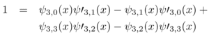
These relationships exist in simpler form at m = 2 with ψ2,0(x) = cos(x)
and ψ2,1(x) = sin(x). For instance,
1 = cos² (x) + sin²(x) (8.17)
= ψ![]() ,0(x) + ψ
,0(x) + ψ![]() ,1(x) (8.18)
,1(x) (8.18)
= ψ2,0(x)ψ![]() 2,1(x) + ψ2,1(x)(−ψ
2,1(x) + ψ2,1(x)(−ψ![]() 2,0(x)) (8.19)
2,0(x)) (8.19)
= ψ2,0(x)ψ![]() 2,1(x) − ψ2,1(x)ψ
2,1(x) − ψ2,1(x)ψ![]() 2,0(x) (8.20)
2,0(x) (8.20)
The same procedure can be pursued for higher m-levels
8.2 Curvature
Equation (3.8) can be thought of as defining a triangle with angle ![]() and magnitude
and magnitude ![]()
Let us define
![]() (8.21)
(8.21)
![]() (8.22)
(8.22)
For fixed x, as m increases ![]() decreases and
decreases and ![]() increases. The triangle
increases. The triangle
becomes longer and narrower.
We can also form a triangle by adding across m-levels the real and imaginary
parts of ![]() If we do so, for positive x the larger m-levels will dominate the summation as x increases, since they grow more rapidly with x. This implies that as x increases, the composite triangle will become more narrow; or, put differently, the angle between the sides of the triangle depends on the length of the sides. This is a characteristic of non-Euclidean geometry.
If we do so, for positive x the larger m-levels will dominate the summation as x increases, since they grow more rapidly with x. This implies that as x increases, the composite triangle will become more narrow; or, put differently, the angle between the sides of the triangle depends on the length of the sides. This is a characteristic of non-Euclidean geometry.
For negative x, as the magnitude of x increases the relative influence of the higher m-levels will decline, because they decrease more rapidly with negative x.
If we view from the perspective of (say) level m = 5, the composite triangle will appear to narrow with increasing positive x, and widen with decreasing negative x. The former corresponds to elliptical geometry, the latter to hyperbolic geometry.
Note that m = 2 provides a perfectly Euclidean geometry.
8.3 The Inner Product on Level m
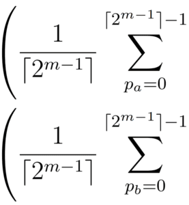
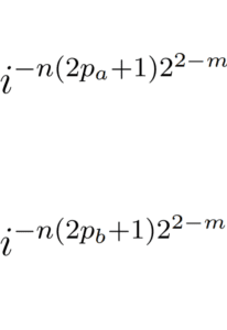
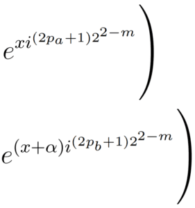
It is possible to compute the inner product at level m with the following equation
(see Appendix F for a derivation).
![]() (8.23)
(8.23)
![]()
![]()
![]()
Here are some examples.
- For m = , Equation (8.24) reduces to
(8.24)
(8.25)
(8.26)
(8.27)
which is simply the familiar rule for adding exponents.
- For m = 1, Equation (8.24) reduces to
(8.32)
(8.33)
(8:34)
(8:35)
(8.36)
This is also familiar, as the dot product of two vectors in a two-dimensional
Euclidean plane.
For m ≥ 3 the inner product becomes more complex, but no less interesting.9 Notice that only for m = 2, corresponding to Euler’s formula, is the inner product independent of x. This is to be expected:10 only for m = 2 does the suitcase term ![]() correspond to a perfect circle, with no growth term.
correspond to a perfect circle, with no growth term.
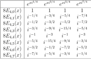
8.4 Differentiation, Rotation and Displacement
Differentiation (or integration), imaginary rotation and displacement are closely
related in Cairns space. We can write
![]() (8.37)
(8.37)
![]() (8.38)
(8.38)
![]() (8.39)
(8.39)
For conciseness, define the displacement
![]() (8.40)
(8.40)
Then
![]()
![]()
![]() (8.41)
(8.41)
So we can think of differentiation as either an imaginary multiplication
(which implies a rotation in the complex plane) or as a shift in the value of
x by ∆m.11 ∆m is a characteristic value of a given m-level. We find
- For m = , ∆0 = 2πi;
- For m = 1, ∆1 = −πi;
- For m = 2, ∆2 = π/2;
- For m = 3, ∆3 = πi¹/²/4;
- For m = 4, ∆4 = πi/8
![]()
![]()
Since
![]() (8.42)
(8.42)
We can equate the two views of differentiation to get
![]()
 (8.43)
Note, however, that the above is a statement about the summation as a
whole, not about particular terms in the summation. In particular, for m ≥ 3
it is not true that12
![]() (8.44)
(8.44)
However, Equation (8.44) is true for m = 2, where it reduces to the familiar
rule that
cos(x) = sin(x + π/2)
8.5 The Roots of nth-Degree Polynomials
It is a singular fact that the equation
a cos(x) − b sin(x) = 0 (8.45)
can be solved simply by rotation.13
To see this, note that if a and b are not both zero, we can write the above
as
![]() (8.46)
(8.46)
for L ≡√a² + b².
![]() and
and ![]() are now in the form of the cos and sin of some angle
are now in the form of the cos and sin of some angle ![]() , defined by
, defined by
cos(![]() ) =
) = ![]() ⇒
⇒ ![]() = arcsin
= arcsin ![]() (8.47)
(8.47)
Or equivalently
sin(![]() ) =
) = ![]() ⇒
⇒ ![]() = arcsin
= arcsin ![]() (8.48)
(8.48)
![]() is the angle formed by a right triangle with sides a and b and hypotenuse L.
is the angle formed by a right triangle with sides a and b and hypotenuse L.
This gives us
L (cos(![]() ) cos(x) − sin(
) cos(x) − sin(![]() ) sin(x)) =
) sin(x)) = ![]() (8.49)
(8.49)
Or
L cos(![]() + x) =
+ x) = ![]() (8.50)
(8.50)
This is a remarkable relationship. It says that any sum of a cos and sin
function with the same period is equal to a single shifted, scaled cos function.
And while it is not clear for what values of x
a cos(x) − b sin(x) = ![]() (8.51)
(8.51)
is true,
L cos(![]() + x) =
+ x) = ![]() (8.52)
(8.52)
obviously holds when x = ±π/2 − ![]() . The roots are found simply by rotating
. The roots are found simply by rotating
by ±π/2 from −![]() .
.
Does a generalization of the above hold for Cairns space generally? If so,
one could imagine solving for the roots of polynomials by projecting onto Cairns
space and performing rotations.
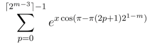
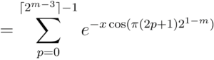
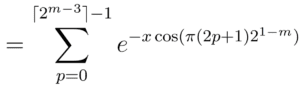
Here is an intriguing special case. From Equation (3.8) we know that the
real and imaginary parts of ![]() are respectively
are respectively
![]() (8.53)
(8.53)
![]() (8.54)
(8.54)
and therefore we have the ratio
![]() (8.55)
(8.55)
From Equation (5.12) we know that ![]() has associated with it a coefficient of
has associated with it a coefficient of ![]() . We may split this into real and imaginary components as
. We may split this into real and imaginary components as
follows.
![]() (8.56)
(8.56)
and therefore, from Equation (5.12), we have
![]() (8.57)
(8.57)
![]() (8.57)
(8.57)
In a sense, ![]() and
and ![]() are the “natural” coefficients of
are the “natural” coefficients of ![]() . For any polynomial consisting of terms at level m
. For any polynomial consisting of terms at level m
with coefficients that are multiples of the natural coefficients, finding roots of
the polynomial is trivial. More explicitly, let
 (8.59)
If there are kR and kI such that
![]() (8.60)
(8.60)
then a solution is 14
![]() (8.61)
(8.61)
One can imagine using the broom theorems, or other means, to collect the projection of a polynomial onto a single level, then distribute it according to the
natural coefficients. However, If there is a general solution to the problem of finding polynomial roots in Cairns space I have not found it as yet, and not for lack of trying. I will not describe here the techniques that do not work, for the enumeration is dismal; and the hand of time is fleeting, and my cigar is burning out.
Chapter 9
Conclusion
But we are not conceived as angels are:
A thousand mindless cares our minds must mar,
Whose troubled tides, through time, turn tyrannous tsar.
In this monograph, the nine characters of the suitcase, ![]() , have been
, have been
unpacked to some sixty pages; and it is clear that we have seen neither the sides
nor the depths of the matter.
There is an interesting debate as to whether mathematics is invented or discovered. On my own experience, I must come down solidly on the side of
discovered. I could not have invented the magic suitcase, simply because it is
much smarter than I am.
I found what I would not have imagined, nor thought possible if imagined,
nor known how to achieve if thought possible. I stumbled across things, very
much like a child at the beach, or (in my better moments) like an archaeologist
carefully excavating a buried palace. I learned mathematics by studying the
suitcase; I taught it nothing.
I have a strong sense of mathematics as existing in a “place”. A place very
different from what we are used to, to be sure, but a place nonetheless. If
one asks if it is a place as real as one on Earth, I would say “more real”. It
existed before our planet was formed, it will exist after the Earth is gone; it is
independent of our universe itself. And it is independent of ourselves as well.
No one can carve their initials in the sides of mathematics.
There is something glorious about learning mathematics, but a kind of sadness as well. I do not fully understand what the suitcase entails, and I very
much suspect that I never will. I am conscious of dimly viewing a garden to
which I can never find the key, and can never be admitted.
’Tis ever and of needs a sorrowful grace
To see a distant beauty, but in trace,
And know it is no work of mortal race.
Appendix A
Derivation of
In Chapter 4, it was stated that by grouping terms with like coefficients of i one
could write the suitcase as
 (A.1)
(A.1)
where
![]() (A.2)
(A.2)
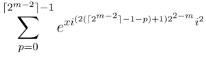
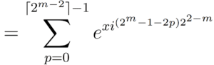
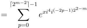
This appendix proves this assertion, by a generalization of the procedure
given in Chapter 4 for m = 2 and m = 3. We proceed by expanding ![]() as Taylor series and grouping terms.
as Taylor series and grouping terms.
 (A.3)
(A.3)
![]() (A.4)
(A.4)
Notice that
![]()
Occurs when
![]() (A.5)
(A.5)
![]() (A.6)
(A.6)
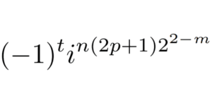
After t ![]() terms the pattern of i exponents will repeat, with sign
terms the pattern of i exponents will repeat, with sign
reversed. Let us call this the “step size”.
Since we are interested in grouping terms with like factors of i, we need to
collect terms that are separated by the step size. This gives us (roughly)
 (A.7)
(A.7)
![]() (A.8)
(A.8)
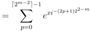
Essentially, we simply define ![]() by the second summation in the above
by the second summation in the above
equation. The one remaining issue is to handle the case m ≤ ![]() correctly, which
correctly, which
corresponds to the function ![]() .
.
Comparison with the Taylor series for ![]() suggests that we change
suggests that we change ![]() . This prevents
. This prevents ![]() from becoming fractional for m ≤ 0, and provides the correct behavior for
from becoming fractional for m ≤ 0, and provides the correct behavior for ![]() . (Of course, the ceiling functions have no effect for m ≥ 1.)
. (Of course, the ceiling functions have no effect for m ≥ 1.)
The second issue for m ≤ 0 is to get the sign right. For m ≤ ![]() the step size
the step size
t ![]() is less than one; the meaning is that the sign never changes.15 We can
is less than one; the meaning is that the sign never changes.15 We can
handle this special case adequately, if not entirely elegantly, by writing
![]() (A.9)
(A.9)
For m ≥ 1 the ![]() factor is simply 1 and has no effect. For m ≤
factor is simply 1 and has no effect. For m ≤ ![]() this
this
factor will be a power of two; since −1 raised to any power of two is 1, this has
the effect of preventing a sign change between terms.16
Appendix B
Proof of the Equivalence of
and
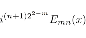
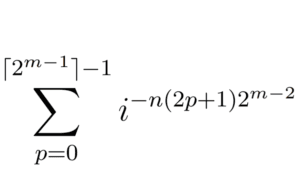
This appendix proves that as claimed by Equation (5.11), the Taylor series view
of the components of ![]() , given by
, given by ![]() , is equivalent to the algebraic
, is equivalent to the algebraic
view of the components given by ![]() .
.
To review, these two views of the suitcase are defined by
![]() (B.1)
(B.1)
![]()
![]()
 (B.2)
(B.2)
Note that it is sufficient to prove the case for ![]() . Since the
. Since the
![]() and
and ![]() can be defined by differentiation (or integration) of
can be defined by differentiation (or integration) of ![]() and
and ![]() respectively, the equivalence of
respectively, the equivalence of ![]() and
and ![]() implies the
implies the
equivalence of all other functions in their respective families. ![]() as a sum of Taylor series, then recursively canceling terms until we are left with
as a sum of Taylor series, then recursively canceling terms until we are left with ![]() .
.
![]()
 (B.3)
(B.3)
![]() (B.4)
(B.4)
where in the last step we expanded the exponential as a Taylor series. Next,
split the series into ![]() overlapping summations, with index n. This gives us
overlapping summations, with index n. This gives us
![]() (B.5)
(B.5)
 (B.6)
(B.6)
![]() (B.7)
(B.7)
![]() (B.8)
(B.8)
For n = ![]() , the term in square brackets becomes
, the term in square brackets becomes
![]() (B.9)
(B.9)
![]() (B.10)
(B.10)
Consequently, for n = 0 we have ![]() =
= ![]() Therefore, to prove it is necessary and sufficient to prove that the terms in square brackets are always zero for n ≥ 1.
Therefore, to prove it is necessary and sufficient to prove that the terms in square brackets are always zero for n ≥ 1.
The terms in square brackets can be written as
![]()
![]()
 (B.11)
Next, split the above summation into two parts, essentially comparing the
first and second quadrants of the complex plane to the third and fourth quadrants. We obtain
![]()
![]() (B.12)
(B.12)
Reparameterizing the second sum gives
![]()
![]() (B.13)
(B.13)
 (B.14)
![]() (B.15)
(B.15)
![]() (B.16)
(B.16)
![]() (B.17)
(B.17)
![]() (B.18)
(B.18)
![]() (B.19)
(B.19)
The two summations differ only by a factor of ![]() : consequently, the sum will be zero for any odd n. For even n, the two sums are equal, so we can rewrite the summation as
: consequently, the sum will be zero for any odd n. For even n, the two sums are equal, so we can rewrite the summation as
 (B.20)
We can again split the summation in two, to compare the first quadrant to
the second quadrant. We find
![]()
![]() (B.21)
(B.21)
Reparameterizing the second summation gives
![]()
![]() (B.22)
(B.22)
![]()
![]() (B.23)
(B.23)
If n contains only a single factor of 2, then ![]() = −1 and the two summations again cancel. Since n cannot be odd and cannot contain a single factor of n, it must contain a factor of 4, in which case the two summations are equal to each other.
= −1 and the two summations again cancel. Since n cannot be odd and cannot contain a single factor of n, it must contain a factor of 4, in which case the two summations are equal to each other.
We can repeat this process as many times as necessary to eliminate the possibility of any n > 0 producing a non-zero sum. In general, this will take m−1 steps, since there ![]() possible values of n and each step eliminates half of the remaining possibilities.
possible values of n and each step eliminates half of the remaining possibilities.
Appendix C
Factoring
This appendix derives Equations (5.39) and (5.42), relating to the factors of ![]() .
.
C.1 Derivation of ![]() Factors
Factors
This section proves Equation (5.39):
![]()
![]() (C.1)
(C.1)
Where we have used the short-hands introduced in Chapter 5:
![]() (C.2)
(C.2)
![]() (C.3)
(C.3)
Equation (C.1) can be derived by a generalization of the procedure given in
Chapter 5 for m = 3.
By definition (see Equation (5.9)) we have
 (C.4)
(C.4)
We can split this summation in two, giving
![]()
![]()
 (C.5)
(C.5)
The general idea is to build cos(x) terms by combining terms between the two
summations. We will then repeat the process to build the cosh(x) terms. To begin, we first reparameterize the second summation.
![]() (C.6)
(C.6)
 (C.7)
(C.7)
Next, we reverse the direction of the second summation, by replacing p with ![]() . This is important because we will want to group the first terms of the first summation with the last terms of the second summation.
. This is important because we will want to group the first terms of the first summation with the last terms of the second summation.
![]()
 (C.8)
(C.8)
Noting that![]() we can write
we can write
 (C.9)
(C.9)
![]() (C.10)
(C.10)
![]() (C.11)
(C.11)
 (C.12)
 (C.13)
 (C.14)
Next, plug back into Equation (C.5) to get
(C.15)
As in Chapter 3, we can use the equation
![]()
to simplify the summation further. We have
![]()
![]()
![]()
![]()
![]()
![]()
![]()
![]()
![]()
![]()
![]()
![]()
Our summation is therefor
![]()
![]()
![]()
The next step is to collapse the ![]()
factors to produce cosh(x). We proceed as above, splitting the series in two,
reparameterizing, reversing direction and grouping terms
![]()
![]()
![]()
![]()
![]()
![]()
Focusing on the second summation for the moment, we find
![]()
![]()
![]()
![]()
![]()
We now reverse the order of summation by substituting ![]() for p.
for p.
Two useful identities are
![]()
![]()
Using these identities, the summation reduces further to
![]()
![]()
Plugging the above back into Equation (C.16), we find
![]()
Collapsing the exponential sum, we have
![]()
![]()
![]()
![]()
As advertised. Equation (C.16) holds for m ≥ 2; for m ≤ 0 we of
course have simply ![]() , and for m = 1 we have
, and for m = 1 we have ![]() .
.
We now know how to express ![]() in terms of the cosh(x) and
in terms of the cosh(x) and
cos(x) functions. Given this, all ![]() can be found by repeated
can be found by repeated
differentiation or integration.
In the next section, we will see another means to compute ![]() .
.
C.2 ![]()
By definition,
![]()
![]()

![]()
![]()
![]()
![]()
Since each integration brings down a factor of ![]() for the
for the ![]() term, we have
term, we have
![]()
![]()
Appendix D
The Orthogonality of
Coefficients
This appendix proves the orthogonality of the vectors defined by
Equation (6.2)
![]()
![]()
(D.1)
for
![]()
That is,
![]() Unless
Unless ![]()
(D.6)
To prove this, we need only consider vector components t in which
both ![]() and
and ![]() have non-zero values. This occurs when t is such
have non-zero values. This occurs when t is such
that
![]()
The first observation is that any two vectors in the same level (i.e., same m-value) are orthogonal. If ![]() then
then ![]() , which says that no two distinct vectors at the same level share any non-zero entries. This is apparent from the table provided in Chapter 5.
, which says that no two distinct vectors at the same level share any non-zero entries. This is apparent from the table provided in Chapter 5.
For ![]() , assume without loss of generality that
, assume without loss of generality that ![]() . Equation (6.2) allows us to break a vector into exactly
. Equation (6.2) allows us to break a vector into exactly ![]() intervals, each with the same pattern of zero and non-zero terms, with only a sign alternation between successive intervals for m >
intervals, each with the same pattern of zero and non-zero terms, with only a sign alternation between successive intervals for m > ![]() . The definition of L ensures that the number of intervals so defined will
. The definition of L ensures that the number of intervals so defined will
be even and ≥ 2.
We note that since ![]() by assumption,
by assumption, ![]() has more intervals than
has more intervals than ![]() , by a factor of
, by a factor of ![]() .
.
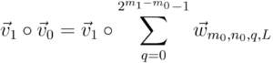
We have the option of expressing ![]() as the sum of
as the sum of ![]() vectors, constructed as follows
vectors, constructed as follows
where
![]()
![]()
(D.10)
The above has the effect of breaking ![]() into a sum of offset vectors, each having the same interval as
into a sum of offset vectors, each having the same interval as ![]() .
. ![]() ◦
◦ ![]() can now be expressed as the sum of the inner products of
can now be expressed as the sum of the inner products of ![]() with each of the
with each of the ![]() . These inner products can be considered separately.
. These inner products can be considered separately.
That is,
 (D.11)
Since each of the ![]() has the same interval length as
has the same interval length as ![]() ,
,![]() ◦ wm0,n0,q,L will have no non-zero terms except when both n0 = n1mod 2m0 (i.e., there are verlapping non-zero terms between
◦ wm0,n0,q,L will have no non-zero terms except when both n0 = n1mod 2m0 (i.e., there are verlapping non-zero terms between ![]() and
and ![]() ) and n1 = n0 + q (i.e., the right decomposition of
) and n1 = n0 + q (i.e., the right decomposition of ![]() ).
).
Thus, proving orthogonality reduces to proving ![]() for
for ![]() mod
mod ![]() and
and ![]() + q, since all other inner products have no common non-zero terms.
+ q, since all other inner products have no common non-zero terms.
Note that ~v1 has an even number of non-zero terms, half of these
+1 and half −1.
![]() has exactly the same positions holding non-zero values as
has exactly the same positions holding non-zero values as ![]() , since both have the same first position for a non-zero term and the same step size. However, while
, since both have the same first position for a non-zero term and the same step size. However, while ![]() has an equal number of positive and negative entries, all entries in
has an equal number of positive and negative entries, all entries in ![]() are of the same sign. This is because the terms of
are of the same sign. This is because the terms of ![]() are pulled from positions of
are pulled from positions of ![]() that are an even number of intervals apart. Therefore,
that are an even number of intervals apart. Therefore, ![]() , which completes the proof that the vectors defined by Equation (6.2) are orthogonal.
, which completes the proof that the vectors defined by Equation (6.2) are orthogonal.
Appendix E
Derivation of the Broom
Theorems
This appendix proves the theorems asserted in Chapter 7, having to
do with translating between levels of Cairns space.
E.1 Sweeping Up
Let![]() and define
and define ![]() By definition,
By definition,
 (E.1)
(E.1)
Let us perform a change of variables
![]()
![]() (E.2)
(E.2)
This creates “big steps” of size ![]() , and covers the terms stepped over with “small steps” of size
, and covers the terms stepped over with “small steps” of size ![]() .As a short-hand, define
.As a short-hand, define
![]()
Then, simply re-expressing the above, we have
![]() (E.3)
(E.3)
Now, switch the order of summation:
![]() (E.4)
(E.4)
The summation
could be expressed at level ![]() if it had a sign alternation of
if it had a sign alternation of ![]() . We can introduce a sign alternation by introducing a factor inside
. We can introduce a sign alternation by introducing a factor inside ![]() that cancels a sign alternation outside
that cancels a sign alternation outside ![]() . This can be done as follows.
. This can be done as follows.
![]() (E.5)
(E.5)
Expanding the definition of q and rearranging, we have
![]()
This gives us what we need. The first factor of the above gives us a sign alternation for Equation (E.4). Since the second factor has no s-dependency it can be moved to the outer (first) summation. Therefore we have
(E.8)
Here ![]() + n plays the role of n at level mv, varying across t. Putting it together, we have
+ n plays the role of n at level mv, varying across t. Putting it together, we have
 (E.9)
(E.9)
![]()
which allows us to express ![]() in terms of functions at level
in terms of functions at level ![]() , for
, for ![]() >
> ![]() ≥
≥ ![]() .
.
E.2 Sweeping Sideways
This section proves Equation (7.3), for expressing a function at level m in terms of other functions at level m.
Let us examine a special case at m = 3 to understand the idea.
From the definition of a Taylor series,
![]()
 (E.14)
![]()

![]()
(E.24)
Notice that in the special case a = ![]() we have
we have ![]() , = 1
, = 1 ![]()
![]()
![]() =
= ![]() and the above reduces to a simple identity.
and the above reduces to a simple identity.
We now apply the same approach more generally.
![]() (E.25)
(E.25)
![]()
(E.26)
Next, take advantage of the properties of derivatives of ![]() ) (see Chapter 4), specifically that
) (see Chapter 4), specifically that ![]() = if n ≥ 1, and
= if n ≥ 1, and ![]() . Consequently, in the first cycle of derivatives in Equation (E.25) the sign will be positive for the first n differentiations, and negative thereafter. This pattern will reverse in the next cycle, and alternate thereafter.
. Consequently, in the first cycle of derivatives in Equation (E.25) the sign will be positive for the first n differentiations, and negative thereafter. This pattern will reverse in the next cycle, and alternate thereafter.
We also know that there are exacly ![]() functions at level m, meaning that after
functions at level m, meaning that after ![]() differentiations we return to the same function, with a sign change.
differentiations we return to the same function, with a sign change.
Combining this information, we have
![]()
![]()
Where, as in Chapter 7 we define whole(n−p) = 1 for (n−p) ≥ 0
and −1 otherwise.
Finally, we note that by the definition of ![]() (see Chapter 4)
(see Chapter 4)
we can write
Appendix F
Derivation of the Inner
Product
This appendix derives Equation (8.24) for the inner product at level m.
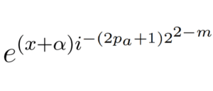
![]() (F.1)
(F.1)
 (F.2)
(F.2)
![]()
 (F.3)
(F.3)
for the inner product at level m.
By definition, the left side of the above is equivalent to
![]()
![]()
![]()
This summation is fairly horrendous. Cats have choked on less. The first order of business is to reverse the order of summations, to temporarily “freeze” the exponent. Otherwise, one is in for a very long night.
Collecting the summations and the coefficients, and bringing the “n” summation to the inside, we obtain
The coefficients depend on n, but the exponents do not. So we can examine the inner summation considering the exponential factor to be constant.
As is often true, it is useful to look at m = 3 explicitly to understand the general pattern. If we look at the factor
![]() (F.4)
(F.4)
for m = 3, we can build the following table showing how it varies with n and p
Since Pa and Pb are fixed for the inner summation, summing over n amounts to multiplying some combination of two columns from the above table together and adding down the rows of those two columns.
It is notable that this procedure will yield zero for all combinations of two columns except (p = 0, p = 3) and (p = 1, p = 2). These happen to be the only combinations for which ![]() .
.
The same pattern holds in the simpler case of m = 2, where the corresponding matrix is
Does this pattern generalize for m ≥ 4?
Let us examine the summation of the coefficients by themselves
 (F.5)
(F.5)
![]() (F.6)
(F.6)
For m ≥ 2 we can split the summation in two:
![]() (F.7)
(F.7)
![]()
![]() (F.8)
(F.8)
![]()
![]() (F.9)
(F.9)
The above summation will be zero whenever pa + pb + 1 is odd, since the second factor will be zero. If Pa + Pb + 1 is even then the second factor reduces to 2. If we assume Pa +Pb + 1 is even then for m ≥ 3 we can again split the summation in two, precisely as above. We obtain
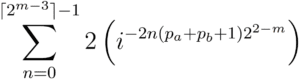
We saw at the previous step that Pa + Pb + 1 must be even for non-zero cases. This step tells us that only even terms which are divisible by four produce a non-zero sum.
We can repeat this process recursively as many times as ![]() can be divided into two equal parts, with at least one member each; that is, m − 1 times. After m − 1 steps, we know that Pa + Pb + 1 must be a multiple of
can be divided into two equal parts, with at least one member each; that is, m − 1 times. After m − 1 steps, we know that Pa + Pb + 1 must be a multiple of ![]() .
.
This provides the generalization of the m = 2 and m = 3 results we saw from the above tables. The summation is now less horrendous. From here, it requires only a cigar and a shot of Pusser’s to complete the derivation of the inner product formula.
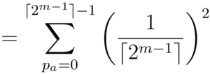
Because we know that only cases where Pa +Pb + 1 = ![]() will have a non-zero sum, we can remove all other cases from the summation without changing the result. Let us therefore define
will have a non-zero sum, we can remove all other cases from the summation without changing the result. Let us therefore define
![]() (F.10)
(F.10)
Which gives
![]()
So
To summarize, we now have the following simplifications available
1. The ummation over n, and the imaginary coefficients, can be replaced by the constraint Pa + Pb + 1 ![]() and a factor of
and a factor of ![]() .
.
2. Since there is only one allowable value of Pb for a given value of Pa, we can eliminate Pb from the exponent and drop the summation over Pb.
This gives us
![]()
![]()
![]()
![]()
![]()
Cancelling and regrouping, we have
Finally, we can rewrite the imaginary sum as follows. In general,
Using this identity for a = ![]() and substituting p for Pa, we have
and substituting p for Pa, we have
![]()
as claimed.
Appendix G
The Cairns Functions For
m ≤ 4
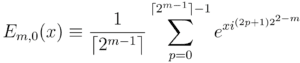
This appendix details ![]() and
and ![]() for the levels m ≤ 4. Recall that
for the levels m ≤ 4. Recall that
![]()
![]() (G.1)
(G.1)
![]() (G.2)
(G.2)
(G.3)
and
 (G.4)
(G.4)
G.1 m ≤ 0
For m = 0,
and
![]()
G.2 m = 1
For m = 1,
and
![]()
G.3 m = 2
For m = 2,
![]()
![]()
G.4 m = 3
For m = 3,
The ![]() values can be found from the below table, generated by integrating
values can be found from the below table, generated by integrating ![]()
![]()
Alternatively, by differentiation of Equation (5.9) we have
![]()
![]()
![]()
![]()
![]()
![]()
G.5 m = 4
For m = 4,
and for ![]() we have
we have
Alternatively, we can differentiate Equation (5.9). For conciseness, we make use of the abbreviations
![]()
![]()
The following identities are also useful for simplifying expressions17
Using the above, we have
![]()
![]()
![]()
![]()
![]()
![]()
![]()
Notice that for even n, ![]() consists of only cosh cos or sinh sin terms, whereas for odd n
consists of only cosh cos or sinh sin terms, whereas for odd n ![]() consists of only cosh sin or sinh cos terms. This is consistent with the requirement that
consists of only cosh sin or sinh cos terms. This is consistent with the requirement that ![]() must be symmetric for even n, and anti-symmetric for odd n.19
must be symmetric for even n, and anti-symmetric for odd n.19
As an exercise, it is possible to use the broom theorems and a modest amount of trickery to show that ![]() = 0 is equivalent to
= 0 is equivalent to
![]()
![]()
An approximate solution is x = 3.76, as is evident from taking a
two-term approximation of ![]() .
.
Refrences
- http://en.wikipedia.org/wiki/Euler%27s formula
- http://www.google.com/patents?vid=USPAT5563556
- This follows from inserting π/2 into Euler’s formula: cos(π/2) = 0 and sin(π/2) = 1, so = cos(π/2) + i sin(π/2) = i.
- The proof of this equation is simply a generalization of the above m = 3 discussion: see Appendix A.
- That is, for even n = and for odd n = −. Thisproperty is familiar from the well-known behavior of and .
- “hypothesize”
- There is a tension between simple exposition, on the one hand, and a certain realism about how results are actually found on the other. In practice, I found the m = 3 relationship by means less than pretty, not suitable for a family monograph, then guessed the general relationship.
- Essentially, the proof amounts to expanding as a sum of Taylor series, then recursively cancelling terms until one is left with . The equivalence for all n follows from parallel differentiation.
- whole is slightly different from the standard sgn function in that whole returns 1 if (n−p) = 0, whereas sgn retuns 0.
- Although notably more difficult to typeset.
- In retrospect, I admit.
- To integrate instead of differentiate, simply reverse the exponent sign of to , and reverse the sign of ∆m.
- see Section 7.3 for the general relationship between functions at a given level.
- Taking the second term to be negative is of course arbitrary, but useful below.
- Incidentally, there is a “hyperbolic dual” in which one uses Equation (3.12) to break the suitcase into hyperbolic, rather than circular, components.
- More precisely, it implies that the sign changes at least twice between adjacent terms, so that by the time one gets to the next term the sign is back where it was.
- In the software industry, this would be known as a “hack”. I prefer the phrase “adequate, if not entirely elegant.”
- These can be derived from the fact that and as can seen by applying the double angle formula starting with .
- The question may arise as to whether it is possible to factor
into a single term, of the form (a + b)(c + d)(e + f).
I believe the answer to be “no”, on symmetry grounds. By inspection,
is invariant under the 7 distinct transforms
Since), it follows that must have the same invariants. For the corresponding 3 transforms essentially map a given element into each of the 3 other elements of But this would not work for , since there are only 5 other elements available for 7 transforms.